bat365 Homepage

Solve Robust Portfolio Maximum Return Problem with Ellipsoidal Uncertainty

This example shows a robust formulation of portfolio optimization with uncertainty in the assets returns. It uses estimateCustomObjectivePortfolio to solve a robust Portfolio problem for a maximum return problem with an ellipsoidal uncertainty. Robust portfolio optimization, in contrast to the deterministic Markowitz mean-variance formulation, considers the uncertainty in the parameters of the problem: the assets' expected returns and their covariance matrix. In the traditional mean-variance model, the mean and covariance are assumed to take the point-values of the historical mean and covariance. However, in robust optimization, the mean and covariance are in a set that contains the most likely realizations, and the problem is optimized with respect to the worst possible outcome in that set.

Define Problem

If the vector of expected returns $r$ has no uncertainty, the portfolio optimization problem that maximizes the returns is

$R_{port} = \max_{x \in X} r^{T} x,$

where

$x \in R^{n}$ is the vector of portfolio weights.
$X$ is the set of feasible allocations represented by a set of constraints.

Robust optimization assumes that the estimates of the expected returns are unreliable, but live in a set that contains the most likely realizations. The set of possible realizations of the expected returns is the uncertainty set and is given by

${r | r \in S (r_{0})},$

where

$S (r_{0})$ is a region around the vector $r_{0}$ .

A common robust formulation of the portfolio problem is the one that tries to maximize the expected return of the portfolio in the worst case scenario of the uncertainty set. This is represented with the following "max-min" problem

$R_{port} = \max_{x \in X} \min_{r \in S (r_{0})} r^{T} x .$

In this example, assume that the uncertainty set follows the common ellipsoidal uncertainty given by

$S (r_{0}) = {r | {(r - r_{0})}^{T} Σ_{r}^{- 1} (r - r_{0}) \leq κ^{2}},$

where

$κ$ is the uncertainty aversion parameter that defines the width of the uncertainty.
$Σ_{r}$ is the covariance matrix of estimation errors in the expected returns $r$ .

Goldfarb and Iyengar [1] show that the robust maximization return problem with ellipsoidal uncertainty in the return is formulated as

$\max_{x \in X} r_{0}^{T} x - κ \sqrt{x^{T} Σ_{r} x} .$

Build Matrix of Estimated Errors in Expected Returns

Assume that the covariance matrix of estimation errors $Σ_{r}$ is a diagonal matrix whose entries are proportional to the assets variance.

Load the data.

% Read the table of daily adjusted close prices for 2006 DJI stocks.
T = readtable('dowPortfolio.xlsx');
% Convert the table to a timetable.
pricesTT = table2timetable(T);
% Remove the DJI stock from the table.
pricesTT = pricesTT(:,2:end);

Build the covariance matrix of estimation errors in the expected returns.

% Compute the returns from the prices.
returnsTT = tick2ret(pricesTT);
% Compute the assets covariance matrix.
Sigma = cov(returnsTT.Variables);
% Compute the covariance matrix of estimation errors in the expected returns.
SigmaR = diag(diag(Sigma));

Solve Robust Problem

Define a Portfolio object.

% Define a traditional mean-variance portfolio.
p = Portfolio;
p = estimateAssetMoments(p,returnsTT,MissingData=true,GetAssetList=true);

Add constraints to the Portfolio object. The portfolio is a fully invested, long-short portfolio with bounds [-0.2,0.2].

% Specify a fully invested constraint.
p = setBudget(p,1,1);
% Specify the long-short bounds.
p = setBounds(p,-0.2,0.2);

Define the objective function with $κ = 0.5$ as the ellipsoidal uncertainty parameter.

% Objective function handle
kappa = 0.5;
robustObjective = @(x) p.AssetMean'*x - kappa*sqrt(x'*SigmaR*x);

Solve the robust maximum return problem using estimateCustomObjectivePortfolio.

wRobustMaxRet = estimateCustomObjectivePortfolio(p,robustObjective,ObjectiveSense="maximize");

Compare Mean-Variance and Robust Portfolio Strategies

Compare the performance of the traditional maximum return portfolio against its robust counterpart using backtesting.

Define the warmup period to compute the initial portfolios for the different strategies using the data in that period.

% Set backtesting warmup period to two 21-day months.
warmupPeriod = 21*2;
% Set a warmup partition of the timetable.
warmupTT = pricesTT(1:warmupPeriod,:);

Compute the initial portfolios using the rebalancing functions (markowitzFcn and robustFcn) that are defined in Local Functions.

% Define the initial Markowitz portfolio.
initialMarkowitz = markowitzFcn(zeros(p.NumAssets,1),warmupTT,p);
% Define the initial robust portfolio.
initialRP = robustFcn(zeros(p.NumAssets,1),warmupTT,p,kappa);

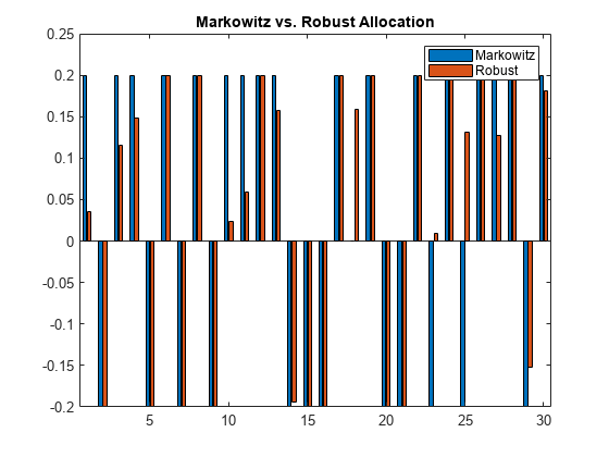
Plot both types of portfolios to compare the initial behavior.

% Plot the intial portfolios.
bar([initialMarkowitz initialRP])
legend('Markowitz','Robust')
title('Markowitz vs. Robust Allocation')

Figure contains an axes object. The axes object with title Markowitz vs. Robust Allocation contains 2 objects of type bar. These objects represent Markowitz, Robust.

Out of 30 assets in the Markowitz allocation, 29 are at the extremes of the feasible bounds. On the other hand, only 17 assets in the robust allocation are at their extremes. The number of assets at the extremes of the feasible bounds shows the sensitivity of the traditional maximum return allocation strategy to the parameters of the problem. The Markowitz strategy invests everything possible in the assets with the highest returns. This result means that the Markowitz strategy shorts the assets with the lowest returns to be able to allocate more to the assets with the largest returns. On the other hand, the robust strategy does not have the same extreme behavior.

Define Backtesting Parameters

Set the backtesting strategies to rebalance every month.

% Define the monthly rebalance frequency.
rebalFreq = 21;

To gather enough data, set the backtestStrategy lookback window for the backtesting to at least 2 months. To remove old data from the parameter estimation, set the lookback window to no more than 6 months.

% Define the lookback window.
lookback = [42 126];

Use a fixed transaction cost equal to 0.5% of the amount traded.

% Define a fixed transaction cost.
transactionCost = 0.005;

Define the allocation strategies using backtestStrategy.

% Define a traditional mean-variance strategy.
stratMarkowitz = backtestStrategy('Markowitz', @(w,TT) markowitzFcn(w,TT,p), ...
    RebalanceFrequency=rebalFreq, ...
    LookbackWindow=lookback, ...
    TransactionCosts=transactionCost, ...
    InitialWeights=initialMarkowitz);

% Define a robust strategy.
stratRobust = backtestStrategy('Robust', @(w,TT) robustFcn(w,TT,p,kappa), ...
    RebalanceFrequency=rebalFreq, ...
    LookbackWindow=lookback, ...
    TransactionCosts=transactionCost, ...
    InitialWeights=initialRP);

Run Backtest

Create a backtestEngine object and then run the backtest using runBacktest.

% Define strategies for backtest engine
strategies = [stratMarkowitz stratRobust];
% Define a backtest engine
backtester = backtestEngine(strategies);
% Run the backtest
backtester = runBacktest(backtester,pricesTT,Start=warmupPeriod);

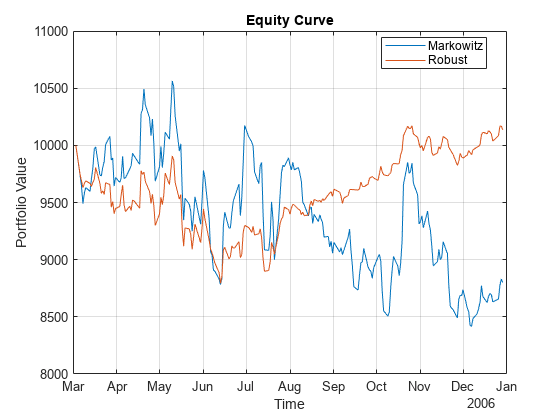
Use equityCurve to plot the equity curve.

equityCurve(backtester)

Figure contains an axes object. The axes object with title Equity Curve, xlabel Time, ylabel Portfolio Value contains 2 objects of type line. These objects represent Markowitz, Robust.

Use summary to generate a table of performance results for both strategies.

summary(backtester)

ans=9×2 table
                        Markowitz       Robust  
                       ___________    __________

    TotalReturn           -0.12004      0.013641
    SharpeRatio           -0.02926      0.011774
    Volatility            0.016383     0.0088013
    AverageTurnover       0.047756      0.021642
    MaxTurnover             1.8849        1.0392
    AverageReturn      -0.00047822    0.00010338
    MaxDrawdown            0.20332       0.12068
    AverageBuyCost           2.276         1.036
    AverageSellCost          2.276         1.036

As expected, the robust strategy has lower volatility than the traditional mean-variance strategy. This characteristic is observed in all the performance indicators that measure variability: volatility, turnover, and maximum drawdown. This result is the expected outcome of robust strategies. Although it is not always the case, in this particular example, the robust strategy also outperforms the traditional mean-variance allocation.

References

[1] Goldfarb, D. and G. Iyengar. "Robust Portfolio Selection Problems." Mathematics of Operations Research. 28(1), pp. 1–38, 2003.

Local Functions

function new_weights = markowitzFcn(~,pricesTT,portObj) 
% Traditional mean-variance portfolio maximum return allocation

% Estimate the portfolio's mean and variance.
p = estimateAssetMoments(portObj,pricesTT,DataFormat='Prices', ...
    MissingData=true);

% Compute the max return portfolio.
new_weights = estimateFrontierLimits(p,'max');

end

function new_weights = robustFcn(~,pricesTT,portObj, ...
    kappa) 
% Robust portfolio maximum return allocation

% Estimate the portfolio's mean and variance.
p = estimateAssetMoments(portObj,pricesTT,DataFormat='Prices', ...
    MissingData=true);

% Cumpute covariance matrix of estimation errors in the expected returns.
SigmaR = diag(diag(p.AssetCovar));

% Define the objective function handle.
robustObjective = @(x) p.AssetMean'*x - kappa*sqrt(x'*SigmaR*x);

% Compute the maximum return portfolio.
new_weights = estimateCustomObjectivePortfolio(p,robustObjective, ...
    ObjectiveSense="maximize");

end

Related Examples

More About

Solver Guidelines for Custom Objective Problems Using Portfolio Objects

Solve Robust Portfolio Maximum Return Problem with Ellipsoidal Uncertainty

Define Problem

Build Matrix of Estimated Errors in Expected Returns

Solve Robust Problem

Compare Mean-Variance and Robust Portfolio Strategies

Define Backtesting Parameters

Run Backtest

References

Local Functions

See Also

Related Examples

More About