Load Portfolio Data

load CAPMuniverse
% Assume that the percentage of women on the board of directors per
% company are as follows
WoB = [0.2857; 0.5; 0.3; 0.2857; 0.3077; 0.2727; ...
    0.4167; 0.2143; 0.3; 0.4167; 0.3077];
table(WoB,'VariableNames',{'WoB'},'RowNames',Assets(1:11))

ans=11×1 table
             WoB  
            ______

    AAPL    0.2857
    AMZN       0.5
    CSCO       0.3
    DELL    0.2857
    EBAY    0.3077
    GOOG    0.2727
    HPQ     0.4167
    IBM     0.2143
    INTC       0.3
    MSFT    0.4167
    ORCL    0.3077

Create Portfolio Object

Create a standard Portfolio object and incorporate the list of assets and estimate the moments of the assets' returns from the data. Use setDefaultConstraints to set the default mean-variance portfolio constraints. These constraints require fully invested, long-only portfolios where the nonnegative weights must sum to 1.

% Create portfolio with default constraints
p = Portfolio('AssetList',Assets(1:11));
p = estimateAssetMoments(p, Data(:,1:11));
p = setDefaultConstraints(p);

Set Group Constraints

Use getGroups to include group contraints. The first group constraint ensures that the weights invested in mixed retail (Amazon and eBay) are at least 15%. The second group constraint ensures that the weights invested in computer companies (Apple, Dell and HP) are between 25% and 50%.

% Group constraints
G = [0 1 0 0 1 0 0 0 0 0 0;
     1 0 0 1 0 0 1 0 0 0 0];
LowG = [0.15; 0.25];
UpG = [Inf; 0.5];
p = setGroups(p, G, LowG, UpG);

Find the minimum and maximum percentage of WoB that a portfolio can attain given these extra group constraints. This is done using the estimateCustomObjectivePortfolio function with the average percentage of women on a company's board as the objective function.

% Set average WoB as the objective
objFun = @(x) WoB'*x;

Find the portfolio with the minimum average percentage of WoB with the group constraints using estimateCustomObjectivePortfolio with the function handle objFun.

% Minimum percetage of women on the board
wgt_minWoB = estimateCustomObjectivePortfolio(p,objFun);
minWoB = objFun(wgt_minWoB)

minWoB = 0.2462

Find the portfolio with the maximum average percentage of WoB with the group constraints using estimateCustomObjectivePortfolio with the name-value argument ObjectiveSense set to maximize.

% Maximum percentage of women on the board
wgt_maxWoB = estimateCustomObjectivePortfolio(p,objFun,...
    ObjectiveSense="maximize");
maxWoB = objFun(wgt_maxWoB)

maxWoB = 0.4792

Compute and Plot the Efficient Surface

Define a grid of WoB percentages such that minWoB $$=$$ targetWoB(1) $$\le \dots \le$$ targetWoB(N) $$=$$ maxWoB.

N = 20; % Size of grid
targetWoB = linspace(minWoB,maxWoB,N);

Use setInequality to set the percentage of WoB as a constraint. The coefficients of the linear constraint should be the WoB percentages associated to each asset, and the right-hand side should be the target portfolio WoB. The convention of the inequality is $$\le$$. Since the goal is to maximize portfolio WoB, then the target WoB should be a lower bound for the portfolio WoB. Therefore, the signs of the coefficients and the right-hand side of the added inequality should be flipped.

Ain = -WoB';
bin = -minWoB; % Start with the smallest WoB
p = setInequality(p,Ain,bin);

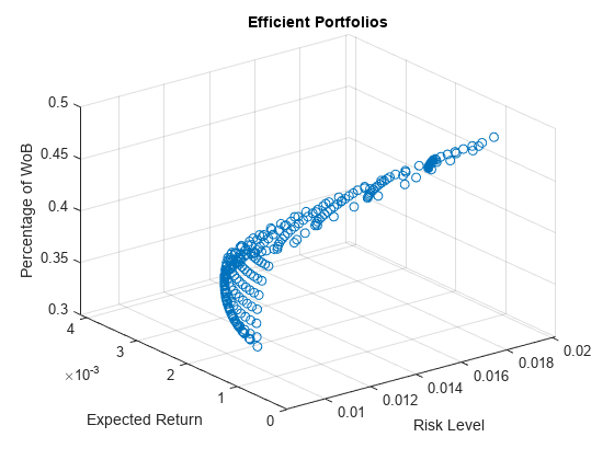
For each target WoB, targetWoB(i), find the efficient mean-variance frontier using estimateFrontier. At each iteration, the right-hand side of the WoB portfolio constraint should be changed to ensure that the returned portfolios achieve at least the target WoB. This method returns the weights of the portfolios on the mean-variance efficient frontier that have a WoB of at least targetWoB(i). Using the weights obtained for each target WoB, compute the portfolios' expected return, risk, and percentage of WoB.

% Get efficient surface values
prsk = cell(N,1);
pret = cell(N,1);
pWoB = cell(N,1);
for i = 1:N
    p.bInequality = -targetWoB(i);
    pwgt = estimateFrontier(p,N);
    [prsk{i},pret{i}] = estimatePortMoments(p,pwgt);
    pWoB{i} = pwgt'*WoB;
end

Plot the efficient portfolios.

% Plot efficient surface
scatter3(cell2mat(prsk),cell2mat(pret),cell2mat(pWoB))
title('Efficient Portfolios')
xlabel('Risk Level')
ylabel('Expected Return')
zlabel('Percentage of WoB')

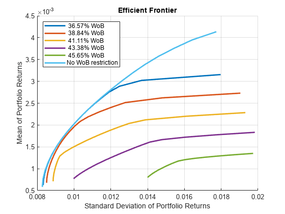
To visualize the tradeoff between a portfolio's average percentage of WoB and the traditional mean-variance efficient frontier, a set of contour plots are computed for some target WoB percentages using the plotContours function in Local Functions.

nC = 5; % Number of contour plots
minContour = max(pWoB{1}); % WoB values lower than this return
                           % overlapped contours.

% Plot contours
plotContours(p,minContour,maxWoB,nC,N)

Exclusion Examples

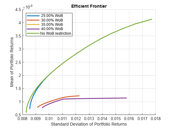
Instead of requiring a specific level for the portfolio's average percentage of WoB, the goal is to find the traditional mean-variance efficient frontiers while excluding assets that have a percentage of WoB lower than a given threshold. You can plot the exclusion using the plotExclusionExample function in Local Functions.

% Remove the average percetage of WoB constraint
p.AInequality = []; p.bInequality = [];

% Set of thresholds for excluding assets
thresholdWoB = 0.25:0.05:0.40;

% Plot exclusion example
plotExclusionExample(p,WoB,thresholdWoB,N)

The differences between this approach and the one presented in the previous section are quite evident. Requiring all the assets to have a WoB percentage of at least 35% gives an efficient frontier that can achieve a return of at most around $1.2{\left(10\right)}^{-3}$. On the other hand, requiring only that the portfolio's average percentage of WoB is 36.57% gives the possibility to reach a return of around $3.2{\left(10\right)}^{-3}$, almost 2.5 times the return obtained when excluding assets. To better show the differences between these two approaches, compute the maximum return achieved for a given standard deviation for the two ways of including the percentage of WoB requirements to the portfolio.

Approach 1

In the first approach, exclude all assets with a WoB percentage lower than 33% and find the portfolio of maximum return that has a standard deviation of at most 0.012.

% Select assets to exclude
ub = zeros(p.NumAssets,1);
ub(WoB >= 0.33) = 1;
p.UpperBound = ub;
% Estimate the return for a risk level of 0.012
pwgt_exclude = estimateFrontierByRisk(p,0.012);
ret_exclude = estimatePortReturn(p,pwgt_exclude)

ret_exclude = 0.0011

% Return constraints to the original portfolio
p.UpperBound = [];

Approach 2

For the second approach, ensure that the average WoB percentage is of at least 33% and find the portfolio of maximum return that has a standard deviation of at most 0.012.

% Include WoB constraint into the portfolio
p = addInequality(p,-WoB',-0.33);
% Estimate the return for a risk level of 0.012
pwgt_avgWoB = estimateFrontierByRisk(p,0.012);
ret_avgWoB = estimatePortReturn(p,pwgt_avgWoB)

ret_avgWoB = 0.0028

% Return constraints to the original portfolio
p.AInequality = []; p.bInequality = [];

Compute the increase in return between these two approaches.

ret_increase = (ret_avgWoB-ret_exclude)/ret_exclude

ret_increase = 1.5202

This ret_increase value shows that the return from the approach that only bounds the portfolio's average WoB percentage instead of excluding certain assets has a return 152% higher (for the same risk level). Hence, when tackling problems with more than two objectives, excluding assets that do not meet a certain criteria might not be the best option. Instead, a weighted sum of the criteria of interest might show better results.

Local Functions

function [] = plotContours(p,minWoB,maxWoB,nContour,nPort)

% Set of WoB levels for contour plot
contourWoB = linspace(minWoB,maxWoB,nContour+1);

% Compute and plot efficient frontier for each value in contourWoB
figure;
hold on
labels = strings(nContour+1,1);
for i = 1:nContour
    p.bInequality = -contourWoB(i);
    plotFrontier(p,nPort);
    labels(i) = sprintf("%6.2f%% WoB",contourWoB(i)*100);
end
% Plot the "original" mean-variance frontier, i.e., the frontier
% without WoB requierements
p.AInequality = []; p.bInequality = [];
plotFrontier(p,nPort);
labels(i+1) = "No WoB restriction";
legend(labels,'Location','northwest')
hold off

end

function [] = plotExclusionExample(p,WoB,thresholdWoB, ...
    nPort)

% Compute and plot efficient frontier excluding assets that are below
% the WoB threshold
nT = length(thresholdWoB);
figure;
hold on
labels = strings(nT+1,1);
for i=1:nT
    ub = zeros(p.NumAssets,1);
    % Only select assets above WoB threshold
    ub(WoB >= thresholdWoB(i)) = 1;
    p.UpperBound = ub;
    plotFrontier(p,nPort);
    labels(i) = sprintf("%6.2f%% WoB",thresholdWoB(i)*100);
end
% Plot the "original" mean-variance frontier, i.e., the frontier
% without the WoB threshold
p.UpperBound = [];
plotFrontier(p,nPort);
labels(i+1) = "No WoB restriction";
legend(labels,'Location','northwest')
hold off

end