bat365 Homepage

Portfolio

Create Portfolio object for mean-variance portfolio optimization and analysis

Description

Use the Portfolio function to create a Portfolio object for mean-variance portfolio optimization.

The main workflow for portfolio optimization is to create an instance of a Portfolio object that completely specifies a portfolio optimization problem and to operate on the Portfolio object using supported functions to obtain and analyze efficient portfolios. For details on this workflow, see Portfolio Object Workflow.

You can use the Portfolio object in several ways. To set up a portfolio optimization problem in a Portfolio object, the simplest syntax is:

p = Portfolio;

This syntax creates a Portfolio object, p, such that all object properties are empty.

The Portfolio object also accepts collections of name-value pair arguments for properties and their values. The Portfolio object accepts inputs for properties with the general syntax:

	p = Portfolio('property1',value1,'property2',value2, ... );

If a Portfolio object exists, the syntax permits the first (and only the first argument) of the Portfolio object to be an existing object with subsequent name-value pair arguments for properties to be added or modified. For example, given an existing Portfolio object in p, the general syntax is:

p = Portfolio(p,'property1',value1,'property2',value2, ... );

Input argument names are not case-sensitive, but must be completely specified. In addition, several properties can be specified with alternative argument names (see Shortcuts for Property Names). The Portfolio object tries to detect problem dimensions from the inputs and, once set, subsequent inputs can undergo various scalar or matrix expansion operations that simplify the overall process to formulate a problem. In addition, a Portfolio object is a value object so that, given portfolio p, the following code creates two objects, p and q, that are distinct:

q = Portfolio(p, ...)

After creating a Portfolio object, you can use the associated object functions to set portfolio constraints, analyze the efficient frontier, and validate the portfolio model.

For more detailed information on the theoretical basis for mean-variance optimization, see Portfolio Optimization Theory.

Creation

Syntax

p = Portfolio

p = Portfolio(Name,Value)

p = Portfolio(p,Name,Value)

Description

example

p = Portfolio creates an empty Portfolio object for mean-variance portfolio optimization and analysis. You can then add elements to the Portfolio object using the supported "add" and "set" functions. For more information, see Creating the Portfolio Object.

example

p = Portfolio(Name,Value) creates a Portfolio object (p) and sets Properties using name-value pairs. For example, p = Portfolio('AssetList',Assets(1:12)). You can specify multiple name-value pairs.

example

p = Portfolio(p,Name,Value) creates a Portfolio object (p) using a previously created Portfolio object p and sets Properties using name-value pairs. You can specify multiple name-value pairs.

Input Arguments

expand all

`p` — Previously constructed Portfolio object
object

Previously constructed Portfolio object, specified using Portfolio.

Properties

expand all

Setting Up the Portfolio Object

`AssetList` — Names or symbols of assets in universe
`[]` (default) | cell array of character vectors | string array

Names or symbols of assets in the universe, specified as a cell array of character vectors or a string array.

Data Types: cell | string

`InitPort` — Initial portfolio
`[]` (default) | vector

Initial portfolio, specified as a vector.

Data Types: double

`Name` — Name for instance of Portfolio object
`[]` (default) | character vector | string

Name for instance of the Portfolio object, specified as a character vector or a string.

Data Types: char | string

`NumAssets` — Number of assets in the universe
`[]` (default) | integer scalar

Number of assets in the universe, specified as an integer scalar.

Data Types: double

Portfolio Object Constraints

`AEquality` — Linear equality constraint matrix
`[]` (default) | matrix

Linear equality constraint matrix, specified as a matrix. For more information, see Linear Equality Constraints.

Data Types: double

`AInequality` — Linear inequality constraint matrix
`[]` (default) | matrix

Linear inequality constraint matrix, specified as a matrix. For more information, see Linear Inequality Constraints.

Data Types: double

`bEquality` — Linear equality constraint vector
`[]` (default) | vector

Linear equality constraint vector, specified as a vector. For more information, see Linear Equality Constraints.

Data Types: double

`bInequality` — Linear inequality constraint vector
`[]` (default) | vector

Linear inequality constraint vector, specified as a vector. For more information, see Linear Inequality Constraints.

Data Types: double

`GroupA` — Group A weights to be bounded by weights in group B
`[]` (default) | matrix

Group A weights to be bounded by weights in group B, specified as a matrix. For more information, see Group Constraints.

Data Types: double

`GroupB` — Group B weights
`[]` (default) | matrix

Group B weights, specified as a matrix. For more information, see Group Constraints.

Data Types: double

`GroupMatrix` — Group membership matrix
`[]` (default) | matrix

Group membership matrix, specified as a matrix. For more information, see Group Ratio Constraints.

Data Types: double

`LowerBound` — Lower-bound constraint
`[]` (default) | vector

Lower-bound constraint, specified as a vector. For more information, see 'Simple' Bound Constraints and 'Conditional' Bound Constraints.

Data Types: double

`LowerBudget` — Lower-bound budget constraint
`[]` (default) | scalar

Lower-bound budget constraint, specified as a scalar. For more information, see Budget Constraints.

Data Types: double

`LowerGroup` — Lower-bound group constraint
`[]` (default) | vector

Lower-bound group constraint, specified as a vector. For more information, see Group Constraints.

Data Types: double

`LowerRatio` — Minimum ratio of allocations between Groups A and B
`[]` (default) | vector

Minimum ratio of allocations between GroupA and GroupB, specified as a vector. For more information, see Group Ratio Constraints.

Data Types: double

`TrackingError` — Upper bound for tracking error constraint
`[]` (default) | scalar

Upper bound for tracking error constraint, specified as a scalar. For more information, see Tracking Error Constraints.

Data Types: double

`TrackingPort` — Tracking portfolio for tracking error constraint
`[]` (default) | vector

Tracking portfolio for tracking error constraint, specified as a vector.

Data Types: double

`UpperBound` — Upper-bound constraint
`[]` (default) | vector

Upper-bound constraint, specified as a vector. For more information, see 'Simple' Bound Constraints and 'Conditional' Bound Constraints.

Data Types: double

`UpperBudget` — Upper-bound budget constraint
`[]` (default) | scalar

Upper-bound budget constraint, specified as a scalar. For more information, see Budget Constraints.

Data Types: double

`UpperGroup` — Upper-bound group constraint
`[]` (default) | vector

Upper-bound group constraint, specified as a vector. For more information, see Group Constraints.

Data Types: double

`UpperRatio` — Maximum ratio of allocations between Groups A and B
`[]` (default) | vector

Maximum ratio of allocations between GroupA and GroupB, specified as a vector. For more information, see Group Ratio Constraints.

Data Types: double

`BoundType` — Type of bounds for each asset weight
`'Simple'` (default) | character vector with value `'Simple'` or `'Conditional'` | string with value `"Simple"` or `"Conditional"` | cell array of character vectors with values `'Simple'` or `'Conditional'` | string array with values `"Simple"` or `"Conditional"`

Type of bounds for each asset weight, specified as a scalar character vector or string, or a cell array of character vectors or a string array. For more information, see setBounds.

Data Types: char | cell | string

`MinNumAssets` — Minimum number of assets allocated in portfolio
`[]` (default) | numeric

Minimum number of assets allocated in portfolio, specified as a scalar numeric value. For more information, see setMinMaxNumAssets and Cardinality Constraints.

Data Types: double

`MaxNumAssets` — Maximum number of assets allocated in portfolio
`[]` (default) | numeric

Maximum number of assets allocated in portfolio, specified as a scalar numeric value. For more information, see setMinMaxNumAssets and Cardinality Constraints.

Data Types: double

`SellTurnover` — Turnover constraint on sales
`[]` (default) | scalar

Turnover constraint on sales, specified as a scalar. For more information, see Average Turnover Constraints and One-Way Turnover Constraints.

Data Types: double

`BuyTurnover` — Turnover constraint on purchases
`[]` (default) | scalar

Turnover constraint on purchases, specified as a scalar. For more information, see Average Turnover Constraints and One-Way Turnover Constraints.

Data Types: double

`Turnover` — Turnover constraint
`[]` (default) | scalar

Turnover constraint, specified as a scalar. For more information, see Average Turnover Constraints and One-Way Turnover Constraints.

Data Types: double

Portfolio Object Modeling

`AssetCovar` — Covariance of asset returns
`[]` (default) | square matrix

Covariance of asset returns, specified as a square matrix.

If AssetCovar is not a symmetric positive semidefinite matrix, use nearcorr to create a positive semidefinite matrix for a correlation matrix.
In some situations, the traditional sample approximation of the covariance matrix performs poorly. An intuitive example is when the number of variables is larger than the number of observations; this results in a noninvertible covariance matrix. Furthermore, because covariance estimation is performed using observations from random data, the estimator contains a certain amount of noise. This noise usually results in ill-conditioned covariance estimates. Working with an ill-conditioned matrix magnifies the impact of estimation errors. You can use covarianceShrinkage and covarianceDenoising for covariance estimation and noise reduction.

Data Types: double

`AssetMean` — Mean of asset returns
`[]` (default) | vector

Mean of asset returns, specified as a vector.

Data Types: double

`BuyCost` — Proportional purchase costs
`[]` (default) | vector

Proportional purchase costs, specified as a vector. For more information, see Net Portfolio Returns.

Data Types: double

`RiskFreeRate` — Risk-free rate
`[]` (default) | scalar

Risk-free rate, specified as a scalar.

Data Types: double

`SellCost` — Proportional sales costs
`[]` (default) | vector

Proportional sales costs, specified as a vector. For more information, see Net Portfolio Returns.

Data Types: double

Object Functions

`setAssetList`	Set up list of identifiers for assets
`setInitPort`	Set up initial or current portfolio
`setDefaultConstraints`	Set up portfolio constraints with nonnegative weights that sum to 1
`getAssetMoments`	Obtain mean and covariance of asset returns from Portfolio object
`setAssetMoments`	Set moments (mean and covariance) of asset returns for Portfolio object
`estimateAssetMoments`	Estimate mean and covariance of asset returns from data
`setCosts`	Set up proportional transaction costs for portfolio
`addEquality`	Add linear equality constraints for portfolio weights to existing constraints
`addGroupRatio`	Add group ratio constraints for portfolio weights to existing group ratio constraints
`addGroups`	Add group constraints for portfolio weights to existing group constraints
`addInequality`	Add linear inequality constraints for portfolio weights to existing constraints
`getBounds`	Obtain bounds for portfolio weights from portfolio object
`getBudget`	Obtain budget constraint bounds from portfolio object
`getCosts`	Obtain buy and sell transaction costs from portfolio object
`getEquality`	Obtain equality constraint arrays from portfolio object
`getGroupRatio`	Obtain group ratio constraint arrays from portfolio object
`getGroups`	Obtain group constraint arrays from portfolio object
`getInequality`	Obtain inequality constraint arrays from portfolio object
`getOneWayTurnover`	Obtain one-way turnover constraints from portfolio object
`setGroups`	Set up group constraints for portfolio weights
`setInequality`	Set up linear inequality constraints for portfolio weights
`setBounds`	Set up bounds for portfolio weights for portfolio
`setBudget`	Set up budget constraints for portfolio
`setCosts`	Set up proportional transaction costs for portfolio
`setEquality`	Set up linear equality constraints for portfolio weights
`setGroupRatio`	Set up group ratio constraints for portfolio weights
`setInitPort`	Set up initial or current portfolio
`setOneWayTurnover`	Set up one-way portfolio turnover constraints
`setTurnover`	Set up maximum portfolio turnover constraint
`setTrackingPort`	Set up benchmark portfolio for tracking error constraint
`setTrackingError`	Set up maximum portfolio tracking error constraint
`setMinMaxNumAssets`	Set cardinality constraints on the number of assets invested in a portfolio
`checkFeasibility`	Check feasibility of input portfolios against portfolio object
`estimateBounds`	Estimate global lower and upper bounds for set of portfolios
`estimateFrontier`	Estimate specified number of optimal portfolios on the efficient frontier
`estimateFrontierByReturn`	Estimate optimal portfolios with targeted portfolio returns
`estimateFrontierByRisk`	Estimate optimal portfolios with targeted portfolio risks
`estimateFrontierLimits`	Estimate optimal portfolios at endpoints of efficient frontier
`plotFrontier`	Plot efficient frontier
`estimateMaxSharpeRatio`	Estimate efficient portfolio to maximize Sharpe ratio for Portfolio object
`estimatePortMoments`	Estimate moments of portfolio returns for Portfolio object
`estimatePortReturn`	Estimate mean of portfolio returns
`estimatePortRisk`	Estimate portfolio risk according to risk proxy associated with corresponding object
`estimateCustomObjectivePortfolio`	Estimate optimal portfolio for user-defined objective function for `Portfolio` object
`setSolver`	Choose main solver and specify associated solver options for portfolio optimization
`setSolverMINLP`	Choose mixed integer nonlinear programming (MINLP) solver for portfolio optimization

Examples

collapse all

Create an Empty Portfolio Object

Open Live Script

You can create a Portfolio object, p, with no input arguments and display it using disp.

p = Portfolio;
disp(p);

  Portfolio with properties:

          BuyCost: []
         SellCost: []
     RiskFreeRate: []
        AssetMean: []
       AssetCovar: []
    TrackingError: []
     TrackingPort: []
         Turnover: []
      BuyTurnover: []
     SellTurnover: []
             Name: []
        NumAssets: []
        AssetList: []
         InitPort: []
      AInequality: []
      bInequality: []
        AEquality: []
        bEquality: []
       LowerBound: []
       UpperBound: []
      LowerBudget: []
      UpperBudget: []
      GroupMatrix: []
       LowerGroup: []
       UpperGroup: []
           GroupA: []
           GroupB: []
       LowerRatio: []
       UpperRatio: []
     MinNumAssets: []
     MaxNumAssets: []
        BoundType: []

This approach provides a way to set up a portfolio optimization problem with the Portfolio function. You can then use the associated set functions to set and modify collections of properties in the Portfolio object.

Create a Portfolio Object Using a Single-Step Setup

Open Live Script

You can use the Portfolio object directly to set up a “standard” portfolio optimization problem, given a mean and covariance of asset returns in the variables m and C.

m = [ 0.05; 0.1; 0.12; 0.18 ];
C = [ 0.0064 0.00408 0.00192 0; 
    0.00408 0.0289 0.0204 0.0119;
    0.00192 0.0204 0.0576 0.0336;
    0 0.0119 0.0336 0.1225 ];

p = Portfolio('assetmean', m, 'assetcovar', C, ...
'lowerbudget', 1, 'upperbudget', 1, 'lowerbound', 0)

p = 
  Portfolio with properties:

          BuyCost: []
         SellCost: []
     RiskFreeRate: []
        AssetMean: [4x1 double]
       AssetCovar: [4x4 double]
    TrackingError: []
     TrackingPort: []
         Turnover: []
      BuyTurnover: []
     SellTurnover: []
             Name: []
        NumAssets: 4
        AssetList: []
         InitPort: []
      AInequality: []
      bInequality: []
        AEquality: []
        bEquality: []
       LowerBound: [4x1 double]
       UpperBound: []
      LowerBudget: 1
      UpperBudget: 1
      GroupMatrix: []
       LowerGroup: []
       UpperGroup: []
           GroupA: []
           GroupB: []
       LowerRatio: []
       UpperRatio: []
     MinNumAssets: []
     MaxNumAssets: []
        BoundType: []

Note that the LowerBound property value undergoes scalar expansion since AssetMean and AssetCovar provide the dimensions of the problem.

Create a Portfolio Object Using a Sequence of Steps

Open Live Script

Using a sequence of steps is an alternative way to accomplish the same task of setting up a “standard” portfolio optimization problem, given a mean and covariance of asset returns in the variables m and C (which also illustrates that argument names are not case sensitive).

m = [ 0.05; 0.1; 0.12; 0.18 ];
C = [ 0.0064 0.00408 0.00192 0; 
    0.00408 0.0289 0.0204 0.0119;
    0.00192 0.0204 0.0576 0.0336;
    0 0.0119 0.0336 0.1225 ];

p = Portfolio;
p = Portfolio(p, 'assetmean', m, 'assetcovar', C);
p = Portfolio(p, 'lowerbudget', 1, 'upperbudget', 1);
p = Portfolio(p, 'lowerbound', 0);
 
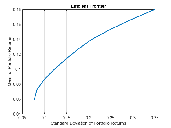
plotFrontier(p);

Figure contains an axes object. The axes object with title Efficient Frontier, xlabel Standard Deviation of Portfolio Returns, ylabel Mean of Portfolio Returns contains an object of type line.

This way works because the calls to Portfolio are in this particular order. In this case, the call to initialize AssetMean and AssetCovar provides the dimensions for the problem. If you were to do this step last, you would have to explicitly dimension the LowerBound property as follows:

m = [ 0.05; 0.1; 0.12; 0.18 ];
C = [ 0.0064 0.00408 0.00192 0; 
    0.00408 0.0289 0.0204 0.0119;
    0.00192 0.0204 0.0576 0.0336;
    0 0.0119 0.0336 0.1225 ];

p = Portfolio;
p = Portfolio(p, 'LowerBound', zeros(size(m)));
p = Portfolio(p, 'LowerBudget', 1, 'UpperBudget', 1);
p = Portfolio(p, 'AssetMean', m, 'AssetCovar', C);
 
plotFrontier(p);

Figure contains an axes object. The axes object with title Efficient Frontier, xlabel Standard Deviation of Portfolio Returns, ylabel Mean of Portfolio Returns contains an object of type line.

If you did not specify the size of LowerBound but, instead, input a scalar argument, the Portfolio object assumes that you are defining a single-asset problem and produces an error at the call to set asset moments with four assets.

Create a Portfolio Object Using Shortcuts for Property Names

Open Live Script

You can create a Portfolio object, p with Portfolio using shortcuts for property names.

m = [ 0.05; 0.1; 0.12; 0.18 ];
C = [ 0.0064 0.00408 0.00192 0; 
    0.00408 0.0289 0.0204 0.0119;
    0.00192 0.0204 0.0576 0.0336;
    0 0.0119 0.0336 0.1225 ];

p = Portfolio('mean', m, 'covar', C, 'budget', 1, 'lb', 0)

p = 
  Portfolio with properties:

          BuyCost: []
         SellCost: []
     RiskFreeRate: []
        AssetMean: [4x1 double]
       AssetCovar: [4x4 double]
    TrackingError: []
     TrackingPort: []
         Turnover: []
      BuyTurnover: []
     SellTurnover: []
             Name: []
        NumAssets: 4
        AssetList: []
         InitPort: []
      AInequality: []
      bInequality: []
        AEquality: []
        bEquality: []
       LowerBound: [4x1 double]
       UpperBound: []
      LowerBudget: 1
      UpperBudget: 1
      GroupMatrix: []
       LowerGroup: []
       UpperGroup: []
           GroupA: []
           GroupB: []
       LowerRatio: []
       UpperRatio: []
     MinNumAssets: []
     MaxNumAssets: []
        BoundType: []

Direct Setting of Portfolio Object Properties

Open Live Script

Although not recommended, you can set properties directly, however no error-checking is done on your inputs.

m = [ 0.05; 0.1; 0.12; 0.18 ];
C = [ 0.0064 0.00408 0.00192 0; 
    0.00408 0.0289 0.0204 0.0119;
    0.00192 0.0204 0.0576 0.0336;
    0 0.0119 0.0336 0.1225 ];

p = Portfolio;
p.NumAssets = numel(m);
p.AssetMean = m;
p.AssetCovar = C;
p.LowerBudget = 1;
p.UpperBudget = 1;
p.LowerBound = zeros(size(m));
disp(p)

  Portfolio with properties:

          BuyCost: []
         SellCost: []
     RiskFreeRate: []
        AssetMean: [4x1 double]
       AssetCovar: [4x4 double]
    TrackingError: []
     TrackingPort: []
         Turnover: []
      BuyTurnover: []
     SellTurnover: []
             Name: []
        NumAssets: 4
        AssetList: []
         InitPort: []
      AInequality: []
      bInequality: []
        AEquality: []
        bEquality: []
       LowerBound: [4x1 double]
       UpperBound: []
      LowerBudget: 1
      UpperBudget: 1
      GroupMatrix: []
       LowerGroup: []
       UpperGroup: []
           GroupA: []
           GroupB: []
       LowerRatio: []
       UpperRatio: []
     MinNumAssets: []
     MaxNumAssets: []
        BoundType: []

Create a `Portfolio` Object and Determine Efficient Portfolios

Open Live Script

Create efficient portfolios:

load CAPMuniverse

p = Portfolio('AssetList',Assets(1:12));
p = estimateAssetMoments(p, Data(:,1:12),'missingdata',true);
p = setDefaultConstraints(p);
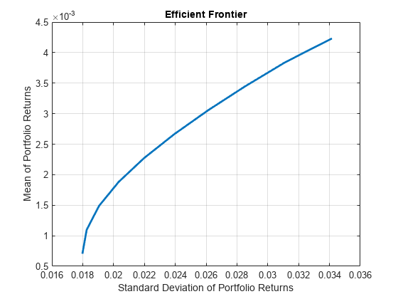
plotFrontier(p);

Figure contains an axes object. The axes object with title Efficient Frontier, xlabel Standard Deviation of Portfolio Returns, ylabel Mean of Portfolio Returns contains an object of type line.

pwgt = estimateFrontier(p, 5);

pnames = cell(1,5);
for i = 1:5
	pnames{i} = sprintf('Port%d',i);
end

Blotter = dataset([{pwgt},pnames],'obsnames',p.AssetList);

disp(Blotter);

            Port1        Port2       Port3       Port4      Port5
    AAPL     0.017926    0.058247    0.097816    0.12955    0    
    AMZN            0           0           0          0    0    
    CSCO            0           0           0          0    0    
    DELL    0.0041906           0           0          0    0    
    EBAY            0           0           0          0    0    
    GOOG      0.16144     0.35678     0.55228    0.75116    1    
    HPQ      0.052566    0.032302    0.011186          0    0    
    IBM       0.46422     0.36045     0.25577    0.11928    0    
    INTC            0           0           0          0    0    
    MSFT      0.29966     0.19222    0.082949          0    0    
    ORCL            0           0           0          0    0    
    YHOO            0           0           0          0    0

Mixed-Integer Mean-Variance Portfolio Optimization Problem

Open Live Script

This example shows how to solve a mean-variance portfolio optimization problem with constraints in the number of selected assets or conditional (semicontinuous) bounds. To solve this problem, you can use a Portfolio object along with different mixed integer nonlinear programming (MINLP) solvers.

Mean-Variance Portfolio

Load the returns data in CAPMuniverse.mat. Then, create a mean-variance Portfolio object with default constraints and a long-only portfolio whose weights sum to 1. For this example, you can define the feasible region of weights $X$ as

$X = {x | \sum_{i = 1}^{n} x_{i} = 1, x_{i} \geq 0} .$

% Load data
load CAPMuniverse.mat

% Create a mean-variance Portfolio object with default constraints
p = Portfolio(AssetList=Assets(1:12));
p = estimateAssetMoments(p,Data(:,1:12));
p = setDefaultConstraints(p);

Include binary variables for this scenario by setting conditional (semicontinuous) bounds. Conditional bounds are those such that $x_{i} = 0$ or $x_{i} \geq ℓ_{i}$ . In this example, $ℓ_{i} = 0.1$ for all assets.

% Set conditional bounds
condLB = 0.1;
condUB = 0.5;
p = setBounds(p,condLB,condUB,BoundType="conditional");

Use estimateFrontier to estimate a set of portfolios on the efficient frontier. The efficient frontier is a curve that shows the trade-off between the return and risk achieved by Pareto-optimal portfolios. For a given return level, the portfolio on the efficient frontier is the one that minimizes the risk while maintaining the desired return. Conversely, for a given risk level, the portfolio on the efficient frontier is the one that maximizes return while maintaining the desired risk level.

% Compute efficient frontier
pwgt = estimateFrontier(p)

pwgt = 12×10

         0         0    0.1000    0.1253    0.1745    0.2236    0.2715    0.3327    0.4111    0.5000
         0         0         0         0         0         0         0         0         0         0
         0         0         0         0         0         0         0         0         0         0
    0.1350         0         0         0         0         0         0         0         0         0
         0         0         0         0         0         0         0         0         0         0
    0.1000    0.1450    0.1406    0.1910    0.2344    0.2778    0.3200    0.3726    0.4415    0.5000
    0.1000    0.1609    0.1642    0.2121    0.2415    0.2709    0.3085    0.2947    0.1474         0
    0.2354    0.1875    0.1290         0         0         0         0         0         0         0
         0         0         0         0         0         0         0         0         0         0
    0.4296    0.4066    0.3662    0.3717    0.2496    0.1277         0         0         0         0
      ⋮

% Compute risk and returns of the portfolios on the efficient frontier
[rsk,ret] = estimatePortMoments(p,pwgt)

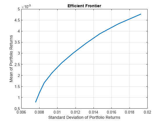
Plot the weights from the frontier estimation using plotFrontier. The resulting curve is piece-wise concave with vertical jumps (discontinuities) between the concave intervals.

% Plot efficient frontier
plotFrontier(p,pwgt)

Figure contains an axes object. The axes object with title Efficient Frontier, xlabel Standard Deviation of Portfolio Returns, ylabel Mean of Portfolio Returns contains an object of type line.

Changing MINLP Solvers

In the previous section, you use the default solver for estimateFrontier. However, you can solve mixed-integer portfolio problems using any of the three algorithms supported by setSolverMINLP: OuterApproximation, ExtendedCP, and TrustRegionCP. Furthermore, the OuterApproximation algorithm accepts an additional name-value argument (ExtendedFormulation) for Portfolo problems, which reformulates problems with quadratic functions to work in an extended space that usually decreases the computation time. All algorithms, including the extended formulation variation of the OuterApproximation algorithm, return the same values within numerical accuracy. The available solvers are:

OuterApproximation — The default algorithm, which is robust and usually faster than ExtenedCP
OuterApproximation with ExtendedFormulation set to true — A robust algorithm that is usually faster than other algorithms, but only supported for Portfolio object problems
ExtendedCP — The most robust solver, but usually the slowest
TrustRegionCP — The fastest algorithm, but one that is less robust and may provide suboptimal solutions

For more information on solvers for mixed-integer portfolio problems, see Choose MINLP Solvers for Portfolio Problems.

To change the MINLP solvers, use setSolverMINLP.

% Select the extended formulation version of 'OuterApproximation'
p_EOA = setSolverMINLP(p,'OuterApproximation',...
    ExtendedFormulation=true);
pwgt_EOA = estimateFrontier(p_EOA);
[rskEOA,retEOA] = estimatePortMoments(p_EOA,pwgt_EOA);

% Select 'TrustRegionCP' as solver
p_TR = setSolverMINLP(p,'TrustRegionCP');
pwgt_TR = estimateFrontier(p_TR);
[rskTR,retTR] = estimatePortMoments(p_TR,pwgt_TR);

% Select 'ExtendedCP' as solver using 'midway' cuts as 'CutGeneration'
p_ECP = setSolverMINLP(p,'ExtendedCP','CutGeneration','midway');
pwgt_ECP = estimateFrontier(p_ECP);
[rskECP,retECP] = estimatePortMoments(p_ECP,pwgt_ECP);

Compare the returns and risks obtained by the portfolios on the efficient frontier from the different solvers. These are same within a numerical accuracy, where the absolute difference is $\leq 10^{- 4}$ .

retTable = table(ret,retEOA,retTR,retECP,...
    'VariableNames',{'OA','EOA','TR','ECP'})

retTable=10×4 table
        OA           EOA            TR           ECP    
    __________    __________    __________    __________

    0.00078336    0.00078336    0.00078334    0.00078348
     0.0012267     0.0012267     0.0012267     0.0012268
       0.00167       0.00167       0.00167     0.0016701
     0.0021133     0.0021133     0.0021133     0.0021134
     0.0025566     0.0025566     0.0025566     0.0025567
     0.0029999     0.0029999     0.0029999         0.003
     0.0034432     0.0034432     0.0034432     0.0034433
     0.0038865     0.0038865     0.0038865     0.0038866
     0.0043298     0.0043298     0.0043298     0.0043299
     0.0047731     0.0047731     0.0047731     0.0047731

rskTable = table(rsk,rskEOA,rskTR,rskECP,...
    'VariableNames',{'OA','EOA','TR','ECP'})

rskTable=10×4 table
       OA           EOA          TR           ECP   
    _________    _________    _________    _________

    0.0075778    0.0075778    0.0075778    0.0075778
    0.0080234    0.0080234    0.0080235    0.0080236
    0.0085488    0.0085488    0.0085488     0.008549
    0.0094024    0.0094024     0.009405    0.0094025
     0.010456     0.010456     0.010456     0.010456
     0.011727     0.011727     0.011776     0.011728
     0.013155     0.013155     0.013155     0.013155
     0.014729     0.014729     0.014729     0.014729
     0.016764     0.016764     0.016764     0.016764
     0.019273     0.019273     0.019273     0.019273

% Compare risks from the different OuterApproximation formulations
norm(rskTable.OA-rskTable.EOA,Inf) <= 1e-4

ans = logical
   1

More About

expand all

Mean-Variance Portfolio Optimization

A mean-variance optimization problem is completely specified with three elements.

The three elements for a mean-variance optimization problem are:

A universe of assets with estimates for the prospective mean and covariance of asset total returns for a period of interest.
A portfolio set that specifies the set of portfolio choices in terms of a collection of constraints.
A model for portfolio return and risk, which, for mean-variance optimization, is either the gross or net mean of portfolio returns and the standard deviation of portfolio returns.

After you specify these three elements in an unambiguous way, you can solve and analyze portfolio optimization problems. The simplest mean-variance portfolio optimization problem has:

A mean and covariance of asset total returns
Nonnegative weights for all portfolios that sum to 1 (the summation constraint is known as a budget constraint)
Built-in models for portfolio return and risk that use the mean and covariance of asset total returns

For more information on the theory and definition of mean-variance optimization supported by portfolio optimization tools in Financial Toolbox™, see Portfolio Optimization Theory.

Portfolio Problem Sufficiency

A mean-variance portfolio optimization is completely specified with the Portfolio object if two condition are met.

The following are the two conditions that must be met:

The moments of asset returns must be specified such that the property AssetMean contains a valid finite mean vector of asset returns and the property AssetCovar contains a valid symmetric positive-semidefinite matrix for the covariance of asset returns.
The first condition is satisfied by setting the properties associated with the moments of asset returns.
The set of feasible portfolios must be a nonempty compact set, where a compact set is closed and bounded.
The second condition is satisfied by an extensive collection of properties that define different types of constraints to form a set of feasible portfolios. Since such sets must be bounded, either explicit or implicit constraints can be imposed, and several functions, such as estimateBounds, provide ways to ensure that your problem is properly formulated.

Given mean and covariance of asset returns in the variables AssetMean and AssetCovar, this problem is completely specified by:

p = Portfolio('AssetMean', AssetMean, 'AssetCovar', AssetCovar,...
'LowerBound', 0, 'UpperBudget',1, 'LowerBudget',1)

or equivalently by:

p = Portfolio;
p = setAssetMoments(p, AssetMean, AssetCovar); 
p = setDefaultConstraints(p);

Although the general sufficiency conditions for mean-variance portfolio optimization go beyond these two conditions, the Portfolio object implemented in Financial Toolbox implicitly handles all these additional conditions. For more information on the Markowitz model for mean-variance portfolio optimization, see Portfolio Optimization.

Shortcuts for Property Names

The Portfolio object has shorter argument names that replace longer argument names associated with specific properties of the Portfolio object.

For example, rather than enter 'assetcovar', the Portfolio object accepts the case-insensitive name 'covar' to set the AssetCovar property in a Portfolio object. Every shorter argument name corresponds with a single property in the Portfolio object. The one exception is the alternative argument name 'budget', which signifies both the LowerBudget and UpperBudget properties. When 'budget' is used, then the LowerBudget and UpperBudget properties are set to the same value to form an equality budget constraint.

Shortcuts for Property Names

Shortcut Argument Name	Equivalent Argument / Property Name
`ae`	`AEquality`
`ai`	`AInequality`
`covar`	`AssetCovar`
`assetnames` or `assets`	`AssetList`
`mean`	`AssetMean`
`be`	`bEquality`
`bi`	`bInequality`
`group`	`GroupMatrix`
`lb`	`LowerBound`
`n` or `num`	`NumAssets`
`rfr`	`RiskFreeRate`
`ub`	`UpperBound`
`budget`	`UpperBudget` and `LowerBudget`

References

[1] For a complete list of references for the Portfolio object, see Portfolio Optimization.

Version History

Introduced in R2011a

Portfolio

Description

Creation

Syntax

Description

Input Arguments

p — Previously constructed Portfolio object object

Properties

Setting Up the Portfolio Object

AssetList — Names or symbols of assets in universe [] (default) | cell array of character vectors | string array

InitPort — Initial portfolio [] (default) | vector

Name — Name for instance of Portfolio object [] (default) | character vector | string

NumAssets — Number of assets in the universe [] (default) | integer scalar

Portfolio Object Constraints

AEquality — Linear equality constraint matrix [] (default) | matrix

AInequality — Linear inequality constraint matrix [] (default) | matrix

bEquality — Linear equality constraint vector [] (default) | vector

bInequality — Linear inequality constraint vector [] (default) | vector

GroupA — Group A weights to be bounded by weights in group B [] (default) | matrix

GroupB — Group B weights [] (default) | matrix

GroupMatrix — Group membership matrix [] (default) | matrix

LowerBound — Lower-bound constraint [] (default) | vector

LowerBudget — Lower-bound budget constraint [] (default) | scalar

LowerGroup — Lower-bound group constraint [] (default) | vector

LowerRatio — Minimum ratio of allocations between Groups A and B [] (default) | vector

TrackingError — Upper bound for tracking error constraint [] (default) | scalar

TrackingPort — Tracking portfolio for tracking error constraint [] (default) | vector

UpperBound — Upper-bound constraint [] (default) | vector

UpperBudget — Upper-bound budget constraint [] (default) | scalar

UpperGroup — Upper-bound group constraint [] (default) | vector

UpperRatio — Maximum ratio of allocations between Groups A and B [] (default) | vector

BoundType — Type of bounds for each asset weight 'Simple' (default) | character vector with value 'Simple' or 'Conditional' | string with value "Simple" or "Conditional" | cell array of character vectors with values 'Simple' or 'Conditional' | string array with values "Simple" or "Conditional"

MinNumAssets — Minimum number of assets allocated in portfolio [] (default) | numeric

MaxNumAssets — Maximum number of assets allocated in portfolio [] (default) | numeric

SellTurnover — Turnover constraint on sales [] (default) | scalar

BuyTurnover — Turnover constraint on purchases [] (default) | scalar

Turnover — Turnover constraint [] (default) | scalar

Portfolio Object Modeling

AssetCovar — Covariance of asset returns [] (default) | square matrix

AssetMean — Mean of asset returns [] (default) | vector

BuyCost — Proportional purchase costs [] (default) | vector

RiskFreeRate — Risk-free rate [] (default) | scalar

SellCost — Proportional sales costs [] (default) | vector

Object Functions

Examples

Create an Empty Portfolio Object

Create a Portfolio Object Using a Single-Step Setup

Create a Portfolio Object Using a Sequence of Steps

Create a Portfolio Object Using Shortcuts for Property Names

Direct Setting of Portfolio Object Properties

Create a Portfolio Object and Determine Efficient Portfolios

Mixed-Integer Mean-Variance Portfolio Optimization Problem

More About

Mean-Variance Portfolio Optimization

Portfolio Problem Sufficiency

Shortcuts for Property Names

References

Version History

See Also

Topics

External Websites

`p` — Previously constructed Portfolio object
object

`AssetList` — Names or symbols of assets in universe
`[]` (default) | cell array of character vectors | string array

`InitPort` — Initial portfolio
`[]` (default) | vector

`Name` — Name for instance of Portfolio object
`[]` (default) | character vector | string

`NumAssets` — Number of assets in the universe
`[]` (default) | integer scalar

`AEquality` — Linear equality constraint matrix
`[]` (default) | matrix

`AInequality` — Linear inequality constraint matrix
`[]` (default) | matrix

`bEquality` — Linear equality constraint vector
`[]` (default) | vector

`bInequality` — Linear inequality constraint vector
`[]` (default) | vector

`GroupA` — Group A weights to be bounded by weights in group B
`[]` (default) | matrix

`GroupB` — Group B weights
`[]` (default) | matrix

`GroupMatrix` — Group membership matrix
`[]` (default) | matrix

`LowerBound` — Lower-bound constraint
`[]` (default) | vector

`LowerBudget` — Lower-bound budget constraint
`[]` (default) | scalar

`LowerGroup` — Lower-bound group constraint
`[]` (default) | vector

`LowerRatio` — Minimum ratio of allocations between Groups A and B
`[]` (default) | vector

`TrackingError` — Upper bound for tracking error constraint
`[]` (default) | scalar

`TrackingPort` — Tracking portfolio for tracking error constraint
`[]` (default) | vector

`UpperBound` — Upper-bound constraint
`[]` (default) | vector

`UpperBudget` — Upper-bound budget constraint
`[]` (default) | scalar

`UpperGroup` — Upper-bound group constraint
`[]` (default) | vector

`UpperRatio` — Maximum ratio of allocations between Groups A and B
`[]` (default) | vector

`MinNumAssets` — Minimum number of assets allocated in portfolio
`[]` (default) | numeric

`MaxNumAssets` — Maximum number of assets allocated in portfolio
`[]` (default) | numeric

`SellTurnover` — Turnover constraint on sales
`[]` (default) | scalar

`BuyTurnover` — Turnover constraint on purchases
`[]` (default) | scalar

`Turnover` — Turnover constraint
`[]` (default) | scalar

`AssetCovar` — Covariance of asset returns
`[]` (default) | square matrix

`AssetMean` — Mean of asset returns
`[]` (default) | vector

`BuyCost` — Proportional purchase costs
`[]` (default) | vector

`RiskFreeRate` — Risk-free rate
`[]` (default) | scalar

`SellCost` — Proportional sales costs
`[]` (default) | vector

Create a `Portfolio` Object and Determine Efficient Portfolios