bat365 Homepage

Backtest Investment Strategies Using Financial Toolbox

Perform backtesting of portfolio strategies using a backtesting framework. Backtesting is a useful tool to compare how investment strategies perform over historical or simulated market data. This example develops five different investment strategies and then compares their performance after running over a one-year period of historical stock data. The backtesting framework is implemented in two Financial Toolbox™ classes: backtestStrategy and backtestEngine.

Load Data

Load one year of adjusted price data for 30 stocks. The backtesting frameworks require adjusted asset prices, meaning prices adjusted for dividends, splits, or other events. The prices must be stored in a MATLAB® timetable with each column holding a time series of asset prices for an investable asset.

For this example, use one year of asset price data from the component stocks of the Dow Jones Industrial Average.

% Read a table of daily adjusted close prices for 2006 DJIA stocks.
T = readtable('dowPortfolio.xlsx');

% For readability, use only 15 of the 30 DJI component stocks.
assetSymbols = ["AA","CAT","DIS","GM","HPQ","JNJ","MCD","MMM","MO","MRK","MSFT","PFE","PG","T","XOM"];

% Prune the table to hold only the dates and selected stocks.
timeColumn = "Dates";
T = T(:,[timeColumn assetSymbols]);

% Convert to the table to a timetable.
pricesTT = table2timetable(T,'RowTimes','Dates');

% View the structure of the prices timetable.
head(pricesTT)

       Dates        AA       CAT      DIS      GM       HPQ      JNJ      MCD      MMM      MO       MRK     MSFT      PFE      PG        T       XOM 
    ___________    _____    _____    _____    _____    _____    _____    _____    _____    _____    _____    _____    _____    _____    _____    _____

    03-Jan-2006    28.72    55.86    24.18    17.82    28.35    59.08    32.72    75.93    52.27    30.73    26.19    22.16    56.38     22.7    56.64
    04-Jan-2006    28.89    57.29    23.77     18.3    29.18    59.99    33.01    75.54    52.65    31.08    26.32    22.88    56.48    22.87    56.74
    05-Jan-2006    29.12    57.29    24.19    19.34    28.97    59.74    33.05    74.85    52.52    31.13    26.34     22.9     56.3    22.92    56.45
    06-Jan-2006    29.02    58.43    24.52    19.61     29.8    60.01    33.25    75.47    52.95    31.08    26.26    23.16    56.24    23.21    57.57
    09-Jan-2006    29.37    59.49    24.78    21.12    30.17    60.38    33.88    75.84    53.11    31.58    26.21    23.16    56.67     23.3    57.54
    10-Jan-2006    28.44    59.25    25.09    20.79    30.33    60.49    33.91    75.37    53.04    31.27    26.35    22.77    56.45    23.16    57.99
    11-Jan-2006    28.05    59.28    25.33    20.61    30.88    59.91     34.5    75.22    53.31    31.39    26.63    23.06    56.65    23.34    58.38
    12-Jan-2006    27.68    60.13    25.41    19.76    30.57    59.63    33.96    74.57    53.23    31.41    26.48     22.9    56.02    23.24    57.77

% View the size of the asset price data set.
numSample = size(pricesTT.Variables, 1);
numAssets = size(pricesTT.Variables, 2);
table(numSample, numAssets)

ans=1×2 table
    numSample    numAssets
    _________    _________

       251          15

Define the Strategies

Investment strategies capture the logic used to make asset allocation decisions while a backtest is running. As the backtest runs, each strategy is periodically given the opportunity to update its portfolio allocation based on the trailing market conditions, which it does by setting a vector of asset weights. The asset weights represent the percentage of available capital invested into each asset, with each element in the weights vector corresponding to the respective column in the asset pricesTT timetable. If the sum of the weights vector is 1, then the portfolio is fully invested.

In this example, there are five backtest strategies. The backtest strategies assign asset weights using the following criteria:

Equal-weighted

$ω EW = (ω_{1}, ω_{2}, . . ., ω_{N}), ω_{i} = \frac{1}{N}$

Maximization of Sharpe ratio

$\underset{ω}{ω SR = argmax} {\frac{r^{'} ω}{\sqrt{ω^{'} Q ω}} | ω \geq 0, \sum_{1}^{N} ω_{i} = 1, 0 \leq ω \leq 0.1}$ , where $r$ is a vector of expected returns and $Q$ is the covariance matrix of asset returns.

Inverse variance

$ω IV =$ $(ω_{1}, ω_{2}, . . ., ω_{N}),$ $ω_{i} = \frac{(σ_{ii}^{- 1})}{\sum_{i = 1}^{N} σ_{ii}^{- 1}}$ , where $σ_{ii}$ are diagonal elements of the asset return covariance matrix.

Markowitz portfolio optimization (maximizing return and minimizing risk with fixed risk-aversion coefficient)

$\underset{}{R_{Mkwtz} = \max_{\underset{}{ω}}} {r^{'} ω - λ ω^{'} Q ω | ω \geq 0, \sum_{1}^{N} ω_{i} = 1, 0 \leq ω \leq 0.1}$ , where $λ$ is the risk-aversion coefficient.

Robust optimization with uncertainty in expected returns
The robust portfolio optimization strategy, in contrast to the deterministic Markowitz formulation, takes into consideration the uncertainty expected returns of the assets and their variances and covariances. Instead of modeling unknown values (for example, expected returns) as one point, typically represented by the mean value calculated from the past, unknowns are specified as a set of values that contain the most likely possible realizations, $r = {r | r \in S (r_{0})}$ .

In this case, the expected return is defined not by the deterministic vector $r_{0}$ but by the region $S (r_{0})$ around the vector $r_{0}$ .

Taking this into consideration, there are several ways to reformulate the portfolio optimization problem. One of the most frequently used methods is to formulate the problem as a problem of finding the maximum and minimum:

$R_{robust} = \max_{ω} \min_{r \in S (r_{0})} {r^{'} ω - λ ω^{'} Q ω | ω \geq 0, \sum_{1}^{N} ω_{i} = 1, 0 \leq ω \leq 0.1}$

In this example, the region of uncertainty $S (r_{0})$ is specified as an ellipsoid:

$S (r_{0}) = {r | (r - r_{0})^{'} Σ_{r}^{- 1} (r - r_{0}) \leq κ^{2}}$

Here, $κ$ - is the uncertainty aversion coefficient that defines how wide the uncertainty region is, and $Σ_{r}$ is the matrix of estimation errors in expected returns $r$ .

With the addition of the ellipsoid uncertainty to the Markowitz model, the robust optimization problem is reformulated as:

$R_{robust} = \max_{ω} {r^{'} ω - λ ω^{'} Q ω - kz | ω \geq 0, {z \geq 0, ω}^{'} Σ_{r} ω - z^{2} \leq 0, \sum_{1}^{N} ω_{i} = 1, 0 \leq ω \leq 0.1}$

Implement the Strategy Rebalance Functions

The core logic of each strategy is implemented in a rebalance function. A rebalance function is a user-defined MATLAB® function that specifies how a strategy allocates capital in a portfolio. The rebalance function is an input argument to backtestStrategy. The rebalance function must implement the following fixed signature:

function new_weights = allocationFunctionName(current_weights, pricesTimetable)

This fixed signature is the API that the backtest framework uses when rebalancing a portfolio. As the backtest runs, the backtesting engine calls the rebalance function of each strategy, passing in these inputs:

current_weights — Current portfolio weights before rebalancing
pricesTimetable — MATLAB® timetable object containing the rolling window of asset prices.

The backtestStrategy rebalance function uses this information to compute the desired new portfolio weights, which are returned to the backtesting engine in the function output new_weights. See the Local Functions sections for the rebalance function for each of the five strategies.

Compute Initial Strategy Weights

Use the strategy rebalance functions to compute the initial weights for each strategy. Setting the initial weights is important because otherwise the strategies begin the backtest with 100% in cash, earning the risk-free rate, until the first rebalance date.

This example uses the first 40 days of the data set (about 2 months) to initialize the strategies. The backtest is then run over the remaining data (about 10 months).

warmupPeriod = 40;

The initial weights are calculated by calling the backtestStrategy rebalance function in the same way that the backtesting engine will call it. To do so, pass in a vector of current weights (all zeros, that is 100% cash) as well as a window of price data that the strategies will use to set the desired weights (the warm-up data partition). Using the rebalance functions to compute the initial weights in this way is not required. The initial weights are a vector of the initial portfolio weights and can be set to any appropriate value. The rebalance functions in this example approximate the state the strategies would be in had they been already running at the start of the backtest.

% No current weights (100% cash position).
current_weights = zeros(1,numAssets);

% Warm-up partition of data set timetable.
warmupTT = pricesTT(1:warmupPeriod,:);

% Compute the initial portfolio weights for each strategy.
equalWeight_initial     = equalWeightFcn(current_weights,warmupTT);
maxSharpeRatio_initial  = maxSharpeRatioFcn(current_weights,warmupTT);
inverseVariance_initial = inverseVarianceFcn(current_weights,warmupTT);
markowitz_initial       = markowitzFcn(current_weights,warmupTT);
robustOptim_initial     = robustOptimFcn(current_weights,warmupTT);

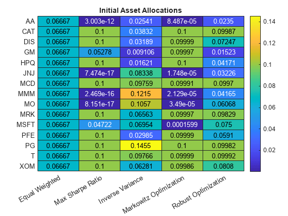
Visualize the initial weight allocations from the strategies.

strategyNames = {'Equal Weighted', 'Max Sharpe Ratio', 'Inverse Variance', 'Markowitz Optimization','Robust Optimization'};
assetSymbols = pricesTT.Properties.VariableNames;
initialWeights = [equalWeight_initial(:), maxSharpeRatio_initial(:), inverseVariance_initial(:), markowitz_initial(:), robustOptim_initial(:)];
heatmap(strategyNames, assetSymbols, initialWeights, 'title','Initial Asset Allocations','Colormap', parula);

Figure contains an object of type heatmap. The chart of type heatmap has title Initial Asset Allocations.

Create Backtest Strategies

To use the strategies in the backtesting framework, you must build backtestStrategy objects, one for each strategy. The backtestStrategy function takes as input the strategy name and rebalancing function for each strategy. Additionally, the backtestStrategy can take a variety of name-value pair arguments to specify various options. For more information on creating backtest strategies, see backtestStrategy.

Set the rebalance frequency and lookback window size are set in terms of number of time steps (that is, rows of the pricesTT timetable). Since the data is daily price data, specify the rebalance frequency and rolling lookback window in days.

% Rebalance approximately every 1 month (252 / 12 = 21).
rebalFreq = 21;

% Set the rolling lookback window to be at least 40 days and at most 126
% days (about 6 months).
lookback  = [40 126];

% Use a fixed transaction cost (buy and sell costs are both 0.5% of amount
% traded).
transactionsFixed = 0.005;

% Customize the transaction costs using a function. See the
% variableTransactionCosts function below for an example.
transactionsVariable = @variableTransactionCosts;

% The first two strategies use fixed transaction costs. The equal-weighted
% strategy does not require a lookback window of trailing data, as its
% allocation is fixed.
strat1 = backtestStrategy('Equal Weighted', @equalWeightFcn, ...
    'RebalanceFrequency', rebalFreq, ...
    'LookbackWindow', 0, ...
    'TransactionCosts', transactionsFixed, ...
    'InitialWeights', equalWeight_initial);

strat2 = backtestStrategy('Max Sharpe Ratio', @maxSharpeRatioFcn, ...
    'RebalanceFrequency', rebalFreq, ...
    'LookbackWindow', lookback, ...
    'TransactionCosts', transactionsFixed, ...
    'InitialWeights', maxSharpeRatio_initial);

% Use variable transaction costs for the remaining strategies.
strat3 = backtestStrategy('Inverse Variance', @inverseVarianceFcn, ...
    'RebalanceFrequency', rebalFreq, ...
    'LookbackWindow', lookback, ...
    'TransactionCosts', @variableTransactionCosts, ...
    'InitialWeights', inverseVariance_initial);

strat4 = backtestStrategy('Markowitz Optimization', @markowitzFcn, ...
    'RebalanceFrequency', rebalFreq, ...
    'LookbackWindow', lookback, ...
    'TransactionCosts', transactionsFixed, ...
    'InitialWeights', markowitz_initial);

strat5 = backtestStrategy('Robust Optimization', @robustOptimFcn, ...
    'RebalanceFrequency', rebalFreq, ...
    'LookbackWindow', lookback, ...
    'TransactionCosts', transactionsFixed, ...
    'InitialWeights', robustOptim_initial);

% Aggregate the strategy objects into an array.
strategies = [strat1, strat2, strat3, strat4, strat5];

Backtest the Strategies

Use the following the workflow to backtest the strategies with a backtestEngine.

Define Backtesting Engine

The backtestEngine function takes as input an array of backtestStrategy objects. Additionally, when using backtestEngine, you can set several options, such as the risk-free rate and the initial portfolio value. When the risk-free rate is specified in annualized terms, the backtestEngine uses Basis property to set the day count convention. For more information on creating backtesting engines, see backtestEngine.

% Risk-free rate is 1% annualized
annualRiskFreeRate = 0.01;

% Create the backtesting engine object
backtester = backtestEngine(strategies, 'RiskFreeRate', annualRiskFreeRate)

backtester = 
  backtestEngine with properties:

               Strategies: [1x5 backtestStrategy]
             RiskFreeRate: 0.0100
           CashBorrowRate: 0
          RatesConvention: "Annualized"
                    Basis: 0
    InitialPortfolioValue: 10000
           DateAdjustment: "Previous"
      PayExpensesFromCash: 0
                NumAssets: []
                  Returns: []
                Positions: []
                 Turnover: []
                  BuyCost: []
                 SellCost: []
         TransactionCosts: []
                     Fees: []

Run Backtest

Use runBacktest to run the backtest using the test data partition. Use the runBacktest name-value pair argument 'Start'to avoid look-ahead bias (that is, "seeing the future"). Begin the backtest at the end of the "warm-up" period. Running the backtest populates the empty fields of the backtestEngine object with the day-by-day backtest results.

backtester = runBacktest(backtester, pricesTT, 'Start', warmupPeriod)

backtester = 
  backtestEngine with properties:

               Strategies: [1x5 backtestStrategy]
             RiskFreeRate: 0.0100
           CashBorrowRate: 0
          RatesConvention: "Annualized"
                    Basis: 0
    InitialPortfolioValue: 10000
           DateAdjustment: "Previous"
      PayExpensesFromCash: 0
                NumAssets: 15
                  Returns: [211x5 timetable]
                Positions: [1x1 struct]
                 Turnover: [211x5 timetable]
                  BuyCost: [211x5 timetable]
                 SellCost: [211x5 timetable]
         TransactionCosts: [1x1 struct]
                     Fees: [1x1 struct]

Examine Backtest Results

Use the summary function to generate a table of strategy performance results for the backtest.

summaryByStrategies = summary(backtester)

summaryByStrategies=9×5 table
                       Equal_Weighted    Max_Sharpe_Ratio    Inverse_Variance    Markowitz_Optimization    Robust_Optimization
                       ______________    ________________    ________________    ______________________    ___________________

    TotalReturn             0.18745            0.14991            0.15906                 0.17404                 0.15655     
    SharpeRatio             0.12559           0.092456            0.12179                 0.10339                 0.11442     
    Volatility            0.0063474          0.0070186          0.0055626               0.0072466               0.0058447     
    AverageTurnover      0.00087623          0.0065762          0.0028666               0.0058268               0.0025172     
    MaxTurnover            0.031251              0.239            0.09114                 0.21873                0.073746     
    AverageReturn        0.00083462         0.00068672          0.0007152              0.00078682              0.00070651     
    MaxDrawdown            0.072392           0.084768           0.054344                0.085544                0.064904     
    AverageBuyCost         0.047298             0.3449            0.15228                  0.3155                  0.1328     
    AverageSellCost        0.047298             0.3449            0.22842                  0.3155                  0.1328

The detailed backtest results, including the daily returns, asset positions, turnover, and fees are stored in properties of the backtestEngine object.

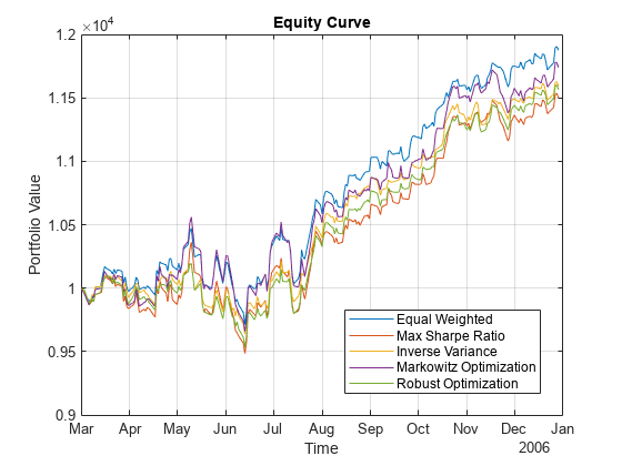
Use equityCurve to plot the equity curve for the five different investment strategies.

equityCurve(backtester)

Figure contains an axes object. The axes object with title Equity Curve, xlabel Time, ylabel Portfolio Value contains 5 objects of type line. These objects represent Equal Weighted, Max Sharpe Ratio, Inverse Variance, Markowitz Optimization, Robust Optimization.

Transposing the summary table to make plots of certain metrics can be useful.

% Transpose the summary table to plot the metrics.
summaryByMetrics = rows2vars(summaryByStrategies);
summaryByMetrics.Properties.VariableNames{1} = 'Strategy'

summaryByMetrics=5×10 table
             Strategy             TotalReturn    SharpeRatio    Volatility    AverageTurnover    MaxTurnover    AverageReturn    MaxDrawdown    AverageBuyCost    AverageSellCost
    __________________________    ___________    ___________    __________    _______________    ___________    _____________    ___________    ______________    _______________

    {'Equal_Weighted'        }      0.18745        0.12559      0.0063474       0.00087623        0.031251       0.00083462       0.072392         0.047298          0.047298    
    {'Max_Sharpe_Ratio'      }      0.14991       0.092456      0.0070186        0.0065762           0.239       0.00068672       0.084768           0.3449            0.3449    
    {'Inverse_Variance'      }      0.15906        0.12179      0.0055626        0.0028666         0.09114        0.0007152       0.054344          0.15228           0.22842    
    {'Markowitz_Optimization'}      0.17404        0.10339      0.0072466        0.0058268         0.21873       0.00078682       0.085544           0.3155            0.3155    
    {'Robust_Optimization'   }      0.15655        0.11442      0.0058447        0.0025172        0.073746       0.00070651       0.064904           0.1328            0.1328

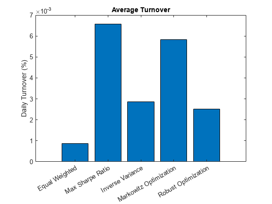
% Compare the strategy turnover.
names = [backtester.Strategies.Name];
nameLabels = strrep(names,'_',' ');
bar(summaryByMetrics.AverageTurnover)
title('Average Turnover')
ylabel('Daily Turnover (%)')
set(gca,'xticklabel',nameLabels)

Figure contains an axes object. The axes object with title Average Turnover, ylabel Daily Turnover (%) contains an object of type bar.

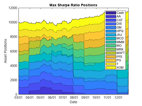
You can visualize the change in the strategy allocations over time using an area chart of the daily asset positions. For information on the assetAreaPlot function, see the Local Functions section.

strategyName = 'Max_Sharpe_Ratio';
assetAreaPlot(backtester,strategyName)

Figure contains an axes object. The axes object with title Max Sharpe Ratio Positions, xlabel Date, ylabel Asset Positions contains 16 objects of type area. These objects represent Cash, AA, CAT, DIS, GM, HPQ, JNJ, MCD, MMM, MO, MRK, MSFT, PFE, PG, T, XOM.

Local Functions

The strategy rebalancing functions as well as the variable transaction cost function follow.

function new_weights = equalWeightFcn(current_weights, pricesTT)
% Equal-weighted portfolio allocation

nAssets = size(pricesTT, 2);
new_weights = ones(1,nAssets);
new_weights = new_weights / sum(new_weights);

end

function new_weights = maxSharpeRatioFcn(current_weights, pricesTT)
% Mean-variance portfolio allocation

nAssets = size(pricesTT, 2);
assetReturns = tick2ret(pricesTT);
% Max 25% into a single asset (including cash)
p = Portfolio('NumAssets',nAssets,...
    'LowerBound',0,'UpperBound',0.1,...
    'LowerBudget',1,'UpperBudget',1);
p = estimateAssetMoments(p, assetReturns{:,:});
new_weights = estimateMaxSharpeRatio(p);

end

function new_weights = inverseVarianceFcn(current_weights, pricesTT) 
% Inverse-variance portfolio allocation

assetReturns = tick2ret(pricesTT);
assetCov = cov(assetReturns{:,:});
new_weights = 1 ./ diag(assetCov);
new_weights = new_weights / sum(new_weights);

end

function new_weights = robustOptimFcn(current_weights, pricesTT) 
% Robust portfolio allocation

nAssets = size(pricesTT, 2);
assetReturns = tick2ret(pricesTT);

Q = cov(table2array(assetReturns));
SIGMAx = diag(diag(Q));

% Robust aversion coefficient
k = 1.1;

% Robust aversion coefficient
lambda = 0.05;

rPortfolio = mean(table2array(assetReturns))';

% Create the optimization problem
pRobust = optimproblem('Description','Robust Portfolio');

% Define the variables
% xRobust - x  allocation vector
xRobust = optimvar('x',nAssets,1,'Type','continuous','LowerBound',0.0,'UpperBound',0.1);
zRobust = optimvar('z','LowerBound',0);

% Define the budget constraint
pRobust.Constraints.budget = sum(xRobust) == 1;

% Define the robust constraint
pRobust.Constraints.robust = xRobust'*SIGMAx*xRobust - zRobust*zRobust <=0;
pRobust.Objective = -rPortfolio'*xRobust + k*zRobust + lambda*xRobust'*Q*xRobust;
x0.x = zeros(nAssets,1);
x0.z = 0;
opt = optimoptions('fmincon','Display','off');
[solRobust,~,~] = solve(pRobust,x0,'Options',opt);
new_weights = solRobust.x;

end

function new_weights = markowitzFcn(current_weights, pricesTT) 
% Robust portfolio allocation

nAssets = size(pricesTT, 2);
assetReturns = tick2ret(pricesTT);

Q = cov(table2array(assetReturns));

% Risk aversion coefficient
lambda = 0.05;

rPortfolio = mean(table2array(assetReturns))';

% Create the optimization problem
pMrkwtz = optimproblem('Description','Markowitz Mean Variance Portfolio ');

% Define the variables
% xRobust - x  allocation vector
xMrkwtz = optimvar('x',nAssets,1,'Type','continuous','LowerBound',0.0,'UpperBound',0.1);

% Define the budget constraint
pMrkwtz.Constraints.budget = sum(xMrkwtz) == 1;

% Define the Markowitz objective
pMrkwtz.Objective = -rPortfolio'*xMrkwtz + lambda*xMrkwtz'*Q*xMrkwtz;
x0.x = zeros(nAssets,1);

opt = optimoptions('quadprog','Display','off');
[solMrkwtz,~,~] = solve(pMrkwtz,x0,'Options',opt);
new_weights = solMrkwtz.x;

end

function [buy, sell] = variableTransactionCosts(deltaPositions)
% Variable transaction cost function
%
% This function is an example of how to compute variable transaction costs.
%
% Compute scaled transaction costs based on the change in market value of
% each asset after a rebalance.  Costs are computed at the following rates:
%
% Buys:
%   $0-$10,000 : 0.5%
%   $10,000+   : 0.35%
% Sells:
%   $0-$1,000  : 0.75%
%   $1,000+    : 0.5%

buy  = zeros(1,numel(deltaPositions));
sell = zeros(1,numel(deltaPositions));

% Buys
idx = 0 < deltaPositions & deltaPositions < 1e4;
buy(idx) = 0.005 * deltaPositions(idx); % 50 basis points
idx = 1e4 <= deltaPositions;
buy(idx) = 0.0035 * deltaPositions(idx); % 35 basis ponits
buy = sum(buy);

% Sells
idx = -1e3 < deltaPositions & deltaPositions < 0;
sell(idx) = 0.0075 * -deltaPositions(idx); % 75 basis points
idx = deltaPositions <= -1e3;
sell(idx) = 0.005 * -deltaPositions(idx); % 50 basis points
sell = sum(sell);

end

function assetAreaPlot(backtester,strategyName)
% Plot the asset allocation as an area plot.

t = backtester.Positions.(strategyName).Time;
positions = backtester.Positions.(strategyName).Variables;
h = area(t,positions);
title(sprintf('%s Positions',strrep(strategyName,'_',' ')));
xlabel('Date');
ylabel('Asset Positions');
datetick('x','mm/dd','keepticks');
xlim([t(1) t(end)])
oldylim = ylim;
ylim([0 oldylim(2)]);
cm = parula(numel(h));
for i = 1:numel(h)
    set(h(i),'FaceColor',cm(i,:));
end
legend(backtester.Positions.(strategyName).Properties.VariableNames)

end