Backtest Investment Strategies with Trading Signals
This example shows how to perform backtesting of portfolio strategies that incorporate investment signals in their trading strategy. The term signals includes any information that a strategy author needs to make with respect to trading decisions outside of the price history of the assets. Such information can include technical indicators, the outputs of machine learning models, sentiment data, macroeconomic data, and so on. This example uses three simple investment strategies based on derivative signal data:
Moving average crossovers
Moving average convergence/divergence
Relative strength index
In this example you can run a backtest using these strategies over one year of stock data. You then analyze the results to compare the performance of each strategy.
Even though technical indicators are not typically used as standalone trading strategies, this example uses these strategies to demonstrate how to build investment strategies based on signal data when you use the backtestEngine object in MATLAB®.
Load Data
Load the adjusted price data for 15 stocks for the year 2006. This example uses a small set of investable assets for readability.
Read a table of daily adjusted close prices for 2006 DJIA stocks.
T = readtable('dowPortfolio.xlsx');For readability, use only 15 of the 30 DJI component stocks.
symbols = ["AA","CAT","DIS","GM","HPQ","JNJ","MCD","MMM","MO","MRK","MSFT","PFE","PG","T","XOM"];
Prune the table to hold only the dates and selected stocks.
timeColumn = "Dates";
T = T(:,[timeColumn symbols]);
Convert the data to a timetable.
pricesTT = table2timetable(T,'RowTimes','Dates');
View the structure of the prices timetable.
head(pricesTT)
       Dates        AA       CAT      DIS      GM       HPQ      JNJ      MCD      MMM      MO       MRK     MSFT      PFE      PG        T       XOM
    ___________    _____    _____    _____    _____    _____    _____    _____    _____    _____    _____    _____    _____    _____    _____    _____

    03-Jan-2006    28.72    55.86    24.18    17.82    28.35    59.08    32.72    75.93    52.27    30.73    26.19    22.16    56.38     22.7    56.64
    04-Jan-2006    28.89    57.29    23.77     18.3    29.18    59.99    33.01    75.54    52.65    31.08    26.32    22.88    56.48    22.87    56.74
    05-Jan-2006    29.12    57.29    24.19    19.34    28.97    59.74    33.05    74.85    52.52    31.13    26.34     22.9     56.3    22.92    56.45
    06-Jan-2006    29.02    58.43    24.52    19.61     29.8    60.01    33.25    75.47    52.95    31.08    26.26    23.16    56.24    23.21    57.57
    09-Jan-2006    29.37    59.49    24.78    21.12    30.17    60.38    33.88    75.84    53.11    31.58    26.21    23.16    56.67     23.3    57.54
    10-Jan-2006    28.44    59.25    25.09    20.79    30.33    60.49    33.91    75.37    53.04    31.27    26.35    22.77    56.45    23.16    57.99
    11-Jan-2006    28.05    59.28    25.33    20.61    30.88    59.91     34.5    75.22    53.31    31.39    26.63    23.06    56.65    23.34    58.38
    12-Jan-2006    27.68    60.13    25.41    19.76    30.57    59.63    33.96    74.57    53.23    31.41    26.48     22.9    56.02    23.24    57.77
Inspect Data Set
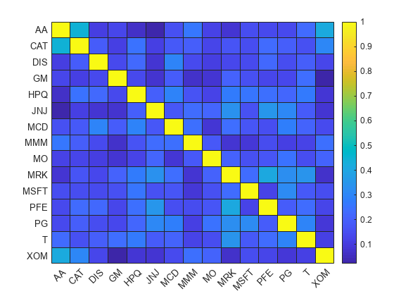
Visualize the correlation and total return of each stock in the data set.
% Visualize the correlation between the 15 stocks.
returns = tick2ret(pricesTT);
stockCorr = corr(returns.Variables);
heatmap(symbols,symbols,stockCorr,'Colormap',parula);
% Visualize the performance of each stock over the range of price data.
totalRet = ret2tick(returns);
plot(totalRet.Dates,totalRet.Variables);
legend(symbols,'Location','NW');
title('Growth of $1 for Each Stock')
ylabel('$')
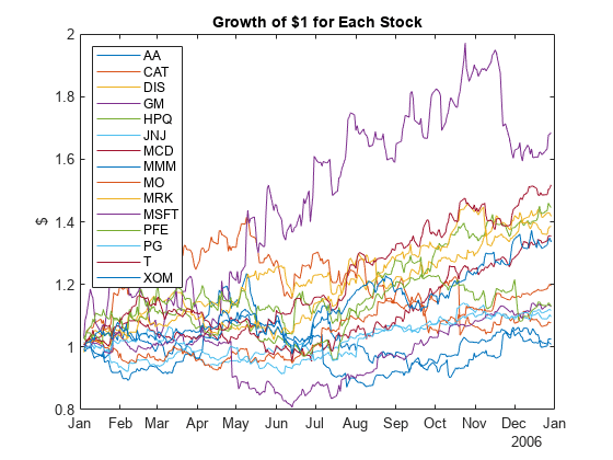
% Get the total return of each stock for the duration of the data set.
totalRet(end,:)ans=1×15 timetable
Dates AA CAT DIS GM HPQ JNJ MCD MMM MO MRK MSFT PFE PG T XOM
___________ ______ ______ ______ ______ ______ ______ ______ ______ ______ ______ ______ ______ ______ ______ _____
29-Dec-2006 1.0254 1.0781 1.4173 1.6852 1.4451 1.0965 1.3548 1.0087 1.1946 1.3856 1.1287 1.1304 1.1164 1.5181 1.336
Build Signal Table
In addition to the historical adjusted asset prices, the backtesting framework allows you to optionally specify signal data when running a backtest. Specify the signal data in a similar way as the prices by using a MATLAB® timetable. The "time" dimension of the signal timetable must match that of the prices timetable — that is, the rows of each table must have matching datetime values for the Time column.
This example builds a signal timetable to support each of the three investment strategies:
Simple moving average crossover (SMA) strategy
Moving Average Convergence / Divergence (MACD) strategy
Relative Strength Index (RSI) strategy
Each strategy has a timetable of signals that are precomputed. Before you run the backtest, you merge the three separate signal timetables into a single aggregate signal timetable to use for the backtest.
SMA: Simple Moving Average Crossover
The SMA indicator uses 5-day and 20-day simple moving averages to make buy and sell decisions. When the 5-day SMA crosses the 20-day SMA (moving upwards), then the stock is bought. When the 5-day SMA crosses below the 20-day SMA, the stock is sold.
% Create SMA timetables using the movavg function.
sma5  = movavg(pricesTT,'simple',5);
sma20 = movavg(pricesTT,'simple',20);
Create the SMA indicator signal timetable.
smaSignalNameEnding = '_SMA5over20';

smaSignal = timetable;
for i = 1:numel(symbols)
    symi = symbols(i);
    % Build a timetable for each symbol, then aggregate them together.
    smaSignali = timetable(pricesTT.Dates,...
        double(sma5.(symi) > sma20.(symi)),...
        'VariableNames',{sprintf('%s%s',symi,smaSignalNameEnding)});
    % Use the synchronize function to merge the timetables together.
    smaSignal = synchronize(smaSignal,smaSignali);
end
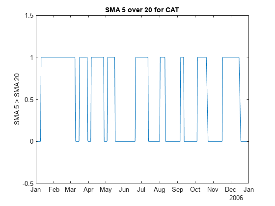
The SMA signal timetable contains an indicator with a value of 1 when the 5-day moving average is above the 20-day moving average for each asset, and a 0 otherwise. The column names for each stock indicator are [stock symbol]SMA5over20. The backtestStrategy object makes trading decisions based on these crossover events.
View the structure of the SMA signal timetable.
head(smaSignal)
       Time        AA_SMA5over20    CAT_SMA5over20    DIS_SMA5over20    GM_SMA5over20    HPQ_SMA5over20    JNJ_SMA5over20    MCD_SMA5over20    MMM_SMA5over20    MO_SMA5over20    MRK_SMA5over20    MSFT_SMA5over20    PFE_SMA5over20    PG_SMA5over20    T_SMA5over20    XOM_SMA5over20
    ___________    _____________    ______________    ______________    _____________    ______________    ______________    ______________    ______________    _____________    ______________    _______________    ______________    _____________    ____________    ______________

    03-Jan-2006          0                0                 0                 0                0                 0                 0                 0                 0                0                  0                 0                 0               0                0
    04-Jan-2006          0                0                 0                 0                0                 0                 0                 0                 0                1                  0                 0                 0               0                0
    05-Jan-2006          0                0                 0                 0                0                 0                 0                 0                 0                0                  0                 0                 0               0                0
    06-Jan-2006          0                0                 0                 0                0                 0                 0                 0                 0                0                  0                 0                 0               0                0
    09-Jan-2006          1                0                 0                 0                1                 0                 0                 0                 0                0                  0                 0                 0               0                0
    10-Jan-2006          1                1                 1                 1                1                 1                 1                 0                 1                1                  1                 1                 1               1                1
    11-Jan-2006          0                1                 1                 1                1                 1                 1                 0                 1                1                  1                 1                 1               1                1
    12-Jan-2006          0                1                 1                 1                1                 1                 1                 0                 1                1                  1                 1                 1               1                1
Plot the signal for a single asset to preview the trading frequency.
plot(smaSignal.Time,smaSignal.CAT_SMA5over20);
ylim([-0.5, 1.5]);
ylabel('SMA 5 > SMA 20');
title(sprintf('SMA 5 over 20 for CAT'));
MACD: Moving Average Convergence/Divergence
You can use the MACD metric in a variety of ways. Often, MACD is compared to its own exponential moving average, but for this example, MACD serves as a trigger for a buy signal when the MACD rises above 0. A position is sold when the MACD falls back below 0.
% Create a timetable of the MACD metric using the MACD function.
macdTT = macd(pricesTT);
Create the MACD indicator signal timetable.
macdSignalNameEnding = '_MACD';

macdSignal = timetable;
for i = 1:numel(symbols)
    symi = symbols(i);
    % Build a timetable for each symbol, then aggregate the symbols together.
    macdSignali = timetable(pricesTT.Dates,...
        double(macdTT.(symi) > 0),...
        'VariableNames',{sprintf('%s%s',symi,macdSignalNameEnding)});
    macdSignal = synchronize(macdSignal,macdSignali);
end
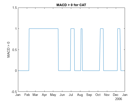
The MACD signal table contains a column for each asset with the name [stock symbol]MACD. Each signal has a value of 1 when the MACD of the stock is above 0. The signal has a value of 0 when the MACD of the stock falls below 0.
head(macdSignal)
       Time        AA_MACD    CAT_MACD    DIS_MACD    GM_MACD    HPQ_MACD    JNJ_MACD    MCD_MACD    MMM_MACD    MO_MACD    MRK_MACD    MSFT_MACD    PFE_MACD    PG_MACD    T_MACD    XOM_MACD
    ___________    _______    ________    ________    _______    ________    ________    ________    ________    _______    ________    _________    ________    _______    ______    ________

    03-Jan-2006       0          0           0           0          0           0           0           0           0          0            0           0           0         0          0
    04-Jan-2006       0          0           0           0          0           0           0           0           0          0            0           0           0         0          0
    05-Jan-2006       0          0           0           0          0           0           0           0           0          0            0           0           0         0          0
    06-Jan-2006       0          0           0           0          0           0           0           0           0          0            0           0           0         0          0
    09-Jan-2006       0          0           0           0          0           0           0           0           0          0            0           0           0         0          0
    10-Jan-2006       0          0           0           0          0           0           0           0           0          0            0           0           0         0          0
    11-Jan-2006       0          0           0           0          0           0           0           0           0          0            0           0           0         0          0
    12-Jan-2006       0          0           0           0          0           0           0           0           0          0            0           0           0         0          0
Similar to the SMA, plot the signal for a single asset to preview the trading frequency.
plot(macdSignal.Time,macdSignal.CAT_MACD)
ylim([-0.5, 1.5]);
ylabel('MACD > 0');
title(sprintf('MACD > 0 for CAT'));
RSI: Relative Strength Index
The RSI is a metric to capture momentum. A common heuristic is to buy when the RSI falls below 30 and to sell when the RSI rises above 70.
rsiSignalNameEnding = '_RSI';

rsiSignal = timetable;
for i = 1:numel(symbols)
    symi = symbols(i);
    rsiValues = rsindex(pricesTT.(symi));
    rsiBuySell = zeros(size(rsiValues));
    rsiBuySell(rsiValues < 30) = 1;
    rsiBuySell(rsiValues > 70) = -1;
    % Build a timetable for each symbol, then aggregate the symbols together.
    rsiSignali = timetable(pricesTT.Dates,...
        rsiBuySell,...
        'VariableNames',{sprintf('%s%s',symi,rsiSignalNameEnding)});
    rsiSignal = synchronize(rsiSignal,rsiSignali);
end
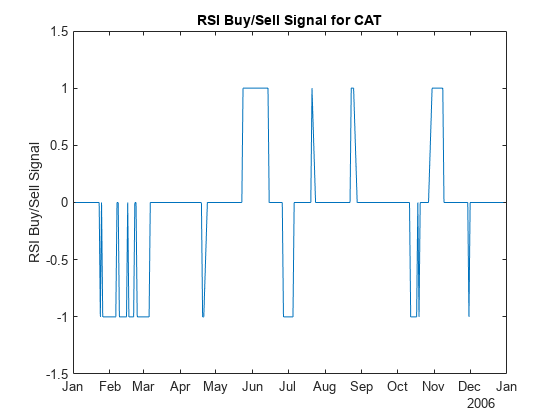
The RSI signal takes a value of 1 (indicating a buy signal) when the RSI value for the stock falls below 30. The signal takes a value of -1 (indicating a sell signal) when the RSI for the stock rises above 70. Otherwise, the signal takes a value of 0, indicating no action.
Plot the signal for a single asset to preview the trading frequency.
plot(rsiSignal.Time,rsiSignal.CAT_RSI)
ylim([-1.5, 1.5]);
ylabel('RSI Buy/Sell Signal');
title(sprintf('RSI Buy/Sell Signal for CAT'));
Build the Strategies
Build the strategies for the backtestStrategy object using the rebalance functions defined in the Local Functions section. Each strategy uses the rebalance function to make trading decisions based on the appropriate signals.
The signals require sufficient trailing data to compute the trading signals (for example, computing the SMA20 for day X requires prices from the 20 days prior to day X). All of the trailing data is captured in the precomputed trading signals. So the actual strategies need only a 2-day lookback window to make trading decisions to evaluate when the signals cross trading thresholds.
All strategies pay 25 basis points transaction costs on buys and sells.
The initial weights are computed based on the signal values after 20 trading days. The backtest begins after this 20 day initialization period.
tradingCosts = 0.0025;

% Use the crossoverRebalanceFunction for both the SMA
% strategy as well as the MACD strategy.  This is because they both trade
% on their respective signals in the same way (buy when signal goes from
% 0->1, sell when signal goes from 1->0).  Build an anonymous
% function for the rebalance functions of the strategies that calls the
% shared crossoverRebalanceFcn() with the appropriate signal name string
% for each strategy.

% Each anonymous function takes the current weights (w), prices (p),
% and signal (s) data from the backtest engine and passes it to the
% crossoverRebalanceFcn function with the signal name string.
smaInitWeights = computeInitialWeights(smaSignal(20,:));
smaRebalanceFcn = @(w,p,s) crossoverRebalanceFcn(w,p,s,smaSignalNameEnding);
smaStrategy = backtestStrategy('SMA',smaRebalanceFcn,...
    'TransactionCosts',tradingCosts,...
    'LookbackWindow',2,...
    'InitialWeights',smaInitWeights);

macdInitWeights = computeInitialWeights(macdSignal(20,:));
macdRebalanceFcn = @(w,p,s) crossoverRebalanceFcn(w,p,s,macdSignalNameEnding);
macdStrategy = backtestStrategy('MACD',macdRebalanceFcn,...
    'TransactionCosts',tradingCosts,...
    'LookbackWindow',2,...
    'InitialWeights',macdInitWeights);

% The RSI strategy uses its signal differently, buying on a 0->1
% transition and selling on a 0->-1 transition.  This logic is captured in
% the rsiRebalanceFcn function defined in the Local Functions section.
rsiInitWeights = computeInitialWeights(rsiSignal(20,:));
rsiStrategy = backtestStrategy('RSI',@rsiRebalanceFcn,...
    'TransactionCosts',tradingCosts,...
    'LookbackWindow',2,...
    'InitialWeights',rsiInitWeights);
Set Up Backtest
As a benchmark, this example also runs a simple equal-weighted strategy to determine if the trading signals are providing valuable insights into future returns of the assets. The benchmark strategy is rebalanced every four weeks.
% The equal weight strategy requires no history, so set LookbackWindow to 0.
benchmarkStrategy = backtestStrategy('Benchmark',@equalWeightFcn,...
    'TransactionCosts',tradingCosts,...
    'RebalanceFrequency',20,...
    'LookbackWindow',0);
Aggregate each of the individual signal timetables into a single backtest signal timetable.
% Combine the three signal timetables.
signalTT = timetable;
signalTT = synchronize(signalTT, smaSignal);
signalTT = synchronize(signalTT, macdSignal);
signalTT = synchronize(signalTT, rsiSignal);
Use backtestEngine to create the backtesting engine and then use runBacktest to run the backtest. The risk-free rate earned on uninvested cash is 1% annualized.
% Put the benchmark strategy and three signal strategies into an array.
strategies = [benchmarkStrategy smaStrategy macdStrategy rsiStrategy];
% Create the backtesting engine.
bt = backtestEngine(strategies,'RiskFreeRate',0.01)
bt =
  backtestEngine with properties:

               Strategies: [1x4 backtestStrategy]
             RiskFreeRate: 0.0100
           CashBorrowRate: 0
          RatesConvention: "Annualized"
                    Basis: 0
    InitialPortfolioValue: 10000
           DateAdjustment: "Previous"
      PayExpensesFromCash: 0
                NumAssets: []
                  Returns: []
                Positions: []
                 Turnover: []
                  BuyCost: []
                 SellCost: []
         TransactionCosts: []
                     Fees: []
Backtest Strategies
% Start with the end of the initial weights calculation warm-up period.
startIdx = 20;

% Run the backtest.
bt = runBacktest(bt,pricesTT,signalTT,'Start',startIdx);
Examine Backtest Results
Use equityCurve to plot the strategy equity curves to visualize their performance over the backtest.
equityCurve(bt)
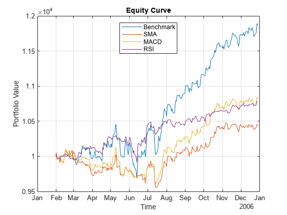
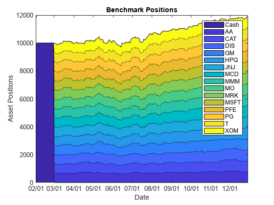
As mentioned previously, these strategies are not typically used as standalone trading signals. In fact, these three strategies perform worse than the simple benchmark strategy for the 2006 timeframe. You can visualize how the strategy allocations change over time using an area chart of the daily asset positions. To do so, use the assetAreaPlot helper function, defined in the Local Functions section.
strategyName = 'Benchmark';
assetAreaPlot(bt,strategyName)
Conclusion
The broad equity market had a very bullish 6 months in the second half of 2006 and all three of these strategies failed to fully capture that growth by leaving too much capital in cash. While none of these strategies performed well on their own, this example demonstrates how you can build signal-based trading strategies and backtest them to assess their performance.
Local Functions
The initial weight calculation function as well as the strategy rebalancing functions follow.
function initial_weights = computeInitialWeights(signals)
% Compute initial weights based on most recent signal.

nAssets = size(signals,2);
final_signal = signals{end,:};
buys = final_signal == 1;
initial_weights = zeros(1,nAssets);
initial_weights(buys) = 1 / nAssets;

end
function new_weights = crossoverRebalanceFcn(current_weights, pricesTT, signalTT, signalNameEnding)
% Signal crossover rebalance function.

% Build cell array of signal names that correspond to the crossover signals.
symbols = pricesTT.Properties.VariableNames;
signalNames = cellfun(@(s) sprintf('%s%s',s,signalNameEnding), symbols, 'UniformOutput', false);

% Pull out the relevant signal data for the strategy.
crossoverSignals = signalTT(:,signalNames);

% Start with our current weights.
new_weights = current_weights;

% Sell any existing long position where the signal has turned to 0.
idx = crossoverSignals{end,:} == 0;
new_weights(idx) = 0;

% Find the new crossovers (signal changed from 0 to 1).
idx = crossoverSignals{end,:} == 1 & crossoverSignals{end-1,:} == 0;

% Bet sizing, split available capital across all remaining assets, and then
% invest only in the new positive crossover assets.  This leaves some
% proportional amount of capital uninvested for future investments into the
% zero-weight assets.
availableCapital = 1 - sum(new_weights);
uninvestedAssets = sum(new_weights == 0);
new_weights(idx) = availableCapital / uninvestedAssets;

end
function new_weights = rsiRebalanceFcn(current_weights, pricesTT, signalTT)
% Buy and sell on 1 and -1 rebalance function.

signalNameEnding = '_RSI';

% Build cell array of signal names that correspond to the crossover signals.
symbols = pricesTT.Properties.VariableNames;
signalNames = cellfun(@(s) sprintf('%s%s',s,signalNameEnding), symbols, 'UniformOutput', false);

% Pull out the relevant signal data for the strategy.
buySellSignals = signalTT(:,signalNames);

% Start with the current weights.
new_weights = current_weights;

% Sell any existing long position where the signal has turned to -1.
idx = buySellSignals{end,:} == -1;
new_weights(idx) = 0;

% Find the new buys (signal is 1 and weights are currently 0).
idx = new_weights == 0 & buySellSignals{end,:} == 1;

% Bet sizing, split available capital across all remaining assets, and then
% invest only in the new positive crossover assets.  This leaves some
% proportional amount of capital uninvested for future investments into the
% zero-weight assets.
availableCapital = 1 - sum(new_weights);
uninvestedAssets = sum(new_weights == 0);
new_weights(idx) = availableCapital / uninvestedAssets;

end
function new_weights = equalWeightFcn(current_weights,~)
% Equal-weighted portfolio allocation.

nAssets = numel(current_weights);
new_weights = ones(1,nAssets);
new_weights = new_weights / sum(new_weights);

end
function assetAreaPlot(backtester,strategyName)
% Plot the asset allocation as an area plot.

t = backtester.Positions.(strategyName).Time;
positions = backtester.Positions.(strategyName).Variables;
h = area(t,positions);
title(sprintf('%s Positions',strrep(strategyName,'_',' ')));
xlabel('Date');
ylabel('Asset Positions');
datetick('x','mm/dd','keepticks');
xlim([t(1) t(end)])
oldylim = ylim;
ylim([0 oldylim(2)]);
cm = parula(numel(h));
for i = 1:numel(h)
    set(h(i),'FaceColor',cm(i,:));
end
legend(backtester.Positions.(strategyName).Properties.VariableNames)

end
See Also
backtestStrategy | backtestEngine | runBacktest | summary
