Analysis and Physics

Physical and empirical relationships form the basis for the throttle and intake manifold dynamics of this model. The air-fuel ratio is computed by dividing the air mass flow rate (pumped from the intake manifold) by the fuel mass flow rate (injected at the valves). The ideal (i.e. stoichiometric) mixture ratio provides a good compromise between power, fuel economy, and emissions. The target air-fuel ratio for this system is 14.6. Typically, a sensor determines the amount of residual oxygen present in the exhaust gas (EGO). This gives a good indication of the mixture ratio and provides a feedback measurement for closed-loop control. If the sensor indicates a high oxygen level, the control law increases the fuel rate. When the sensor detects a fuel-rich mixture, corresponding to a very low level of residual oxygen, the controller decreases the fuel rate.

Modeling

Figure 1 shows the top level of the Simulink model. To open the model, click Open Model. Press the Play button in the model window toolbar to run the simulation. The model loads necessary data into the model workspace from sldemo_fuelsys_data.m. The model logs relevant data to MATLAB workspace in a data structure called sldemo_fuelsys_output and streams the data to the Simulation Data Inspector. Logged signals are marked with a blue indicator while streaming signals are marked with the light blue badge (see Figure 1).

Note that loading initial conditions into the model workspace keeps simulation data isolated from data in other open models that you may have open. This also helps avoid MATLAB workspace cluttering. To view the contents of the model workspace select Modeling > Model Explorer, and click on Model Workspace from the Model Hierarchy list.

Notice that units are visible on the model and subsystem icons and signal lines. Units are specified on the ports and on the bus object.

Figure 1: Top-level diagram for the fuel control system model

The Dashboard subsystem (shown in Figure 2) allows you to interact with the model during simulation. The Fault Injection switches can be moved from the Normal to Fail position to simulate sensor failures, while the Engine Speed selector switch can be toggled to change the engine speed. The fuel and air/fuel ratio signals are visualized using the dashboard gauges and scopes to provide visual feedback during a simulation run.

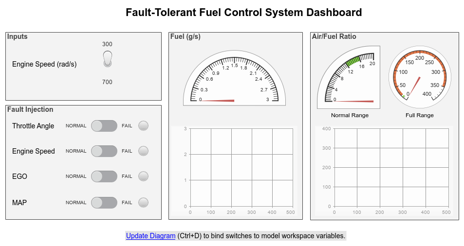
Figure 2: Dashboard subsystem for the fuel control system model

The fuel_rate_control uses signals from the system's sensors to determine the fuel rate which gives a stoichiometric mixture. The fuel rate combines with the actual air flow in the engine gas dynamics model to determine the resulting mixture ratio as sensed at the exhaust.

You can selectively disable each of the four sensors (throttle angle, speed, EGO and manifold absolute pressure [MAP]) by using the slider switches in the dashboard subsystem, to simulate failures. Simulink accomplishes this by binding slider switches to the value parameter of the constant block. Double-click on the dashboard subsystem to open the control dashboard to change the position of the switch. Similarly, you can induce the failure condition of a high engine speed by toggling the engine speed switch on the dashboard subsystem. A Repeating Table block provides the throttle angle input and periodically repeats the sequence of data specified in the mask.

The fuel_rate_control block, shown in Figure 3, uses the sensor input and feedback signals to adjust the fuel rate to give a stoichiometric ratio. The model uses three subsystems to implement this strategy: control logic, airflow calculation, and fuel calculation. Under normal operation, the model estimates the airflow rate and multiplies the estimate by the reciprocal of the desired ratio to give the fuel rate. Feedback from the oxygen sensor provides a closed-loop adjustment of the rate estimation in order to maintain the ideal mixture ratio.

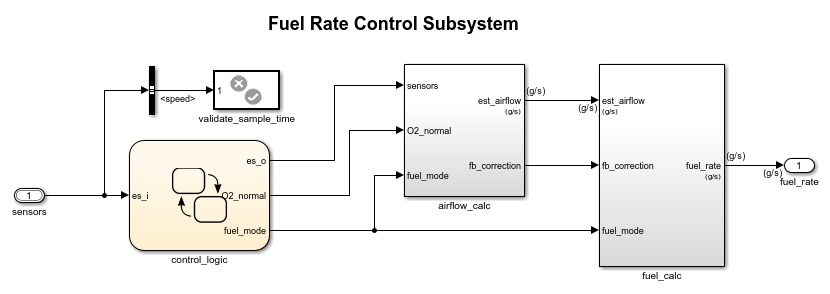
Figure 3: Fuel rate controller subsystem

Control Logic

A single Stateflow chart, consisting of a set of six parallel states, implements the control logic in its entirety. The four parallel states shown at the top of Figure 4 correspond to the four individual sensors. The remaining two parallel states at the bottom consider the status of the four sensors simultaneously and determine the overall system operating mode. The model synchronously calls the entire Stateflow diagram at a regular sample time interval of 0.01 sec. This permits the conditions for transitions to the correct mode to be tested on a timely basis.

To open the control_logic Stateflow chart, double-click on it in the fuel_rate_control subsystem.

Figure 4: The control logic chart

When execution begins, all of the states start in their normal mode with the exception of the oxygen sensor (EGO). The O2_warmup state is entered initially until the warmup period is complete. The system detects throttle and pressure sensor failures when their measured values fall outside their nominal ranges. A manifold vacuum in the absence of a speed signal indicates a speed sensor failure. The oxygen sensor also has a nominal range for failure conditions but, because zero is both the minimum signal level and the bottom of the range, failure can be detected only when it exceeds the upper limit.

Regardless of which sensor fails, the model always generates the directed event broadcast Fail.INC. In this way the triggering of the universal sensor failure logic is independent of the sensor. The model also uses a corresponding sensor recovery event, Fail.DEC. The Fail state keeps track of the number of failed sensors. The counter increments on each Fail.INC event and decrements on each Fail.DEC event. The model uses a superstate, Multi, to group all cases where more than one sensor has failed.

The bottom parallel state represents the fueling mode of the engine. If a single sensor fails, operation continues but the air/fuel mixture is richer to allow smoother running at the cost of higher emissions. If more than one sensor has failed, the engine shuts down as a safety measure, since the air/fuel ratio cannot be controlled reliably.

During the oxygen sensor warm-up, the model maintains the mixture at normal levels. If this is unsatisfactory, you can change the design by moving the warm-up state to within the Rich_Mixture superstate. If a sensor failure occurs during the warm-up period, the Single_Failure state is entered after the warm-up time elapses. Otherwise, the Normal state is activated at this time.

A protective overspeed feature has been added to the model by creating a new state in the Fuel_Disabled superstate. Through the use of history junctions, we assured that the chart returns to the appropriate state when the model exits the overspeed state. As the safety requirements for the engine become better specified, we can add additional shutdown states to the Fuel_Disabled superstate.

Sensor Correction

When a sensor fails, the model computes an estimate of the sensor. For example, open the pressure sensor calculation. Under normal sensor operation, the model uses the value of the pressure sensor. Otherwise, the model estimates the value.

The model computes an estimate of manifold pressure as a function of the engine speed and throttle position. To compute the value, the model uses a Simulink function inside Stateflow.

Airflow Calculation

The Airflow Calculation block (shown in Figure 6) is the location for the central control laws. This block is found inside the fuel_rate_control subsystem (open this block). The block estimates the intake air flow to determine the fuel rate which gives the appropriate air/fuel ratio. Closed-loop control adjusts the estimation according to the residual oxygen feedback in order to maintain the mixture ratio precisely. Even when a sensor failure mandates open-loop operation, the most recent closed-loop adjustment is retained to best meet the control objectives.

Figure 6: Airflow estimation and correction

Equation 1

The engine's intake air flow can be formulated as the product of the engine speed, the manifold pressure and a time-varying scale factor.

Cpump is computed by a lookup table and multiplied by the speed and pressure to form the initial flow estimate. During transients, the throttle rate, with the derivative approximated by a high-pass filter, corrects the air flow for filling dynamics. The control algorithm provides additional correction according to Equation 2.

Equation 2

Figure 7: Engine Gas Dynamics subsystem

Figure 8: Mixing & Combustion block within the Engine Gas Dynamics subsystem

The nonlinear oxygen sensor (EGO Sensor block) is found inside the Mixing & Combustion block (see Figure 8) within the Engine Gas Dynamics subsystem (see Figure 7). EGO Sensor is modeled as a hyperbolic tangent function, and it provides a meaningful signal when in the vicinity of 0.5 volt. The raw error in the feedback loop is thus detected with a switching threshold, as indicated in Equation 2. If the air-fuel ratio is low (the mixture is lean), the original air estimate is too small and needs to be increased. Conversely, when the oxygen sensor output is high, the air estimate is too large and needs to be decreased. Integral control is utilized so that the correction term achieves a level that brings about zero steady-state error in the mixture ratio.

The normal closed-loop operation mode, LOW, adjusts the integrator dynamically to minimize the error. The integration is performed in discrete time, with updates every 10 milliseconds. When operating open-loop however, in the RICH or O2 failure modes, the feedback error is ignored and the integrator is held. This gives the best correction based on the most recent valid feedback.

Fuel Calculation

The fuel_calc subsystem (within the fuel_rate_control subsystem, see Figure 9) sets the injector signal to match the given airflow calculation and fault status. The first input is the computed airflow estimation. This is multiplied with the target fuel/air ratio to get the commanded fuel rate. Normally the target is stoichiometric, i.e. equals the optimal air to fuel ratio of 14.6. When a sensor fault occurs, the Stateflow control logic sets the mode input to a value of 2 or 3 (RICH or DISABLED) so that the mixture is either slightly rich of stoichiometric or is shut down completely.

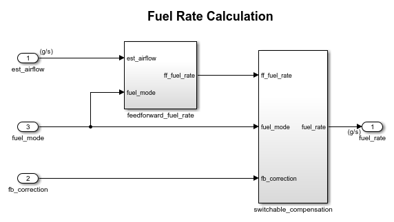
Figure 9: fuel_calc subsystem

The fuel_calc subsystem (Figure 9) employs adjustable compensation (Figure 10) in order to achieve different purposes in different modes. In normal operation, phase lead compensation of the feedback correction signal adds to the closed-loop stability margin. In RICH mode and during EGO sensor failure (open loop), however, the composite fuel signal is low-pass filtered to attenuate noise introduced in the estimation process. The end result is a signal representing the fuel flow rate which, in an actual system, would be translated to injector pulse times.

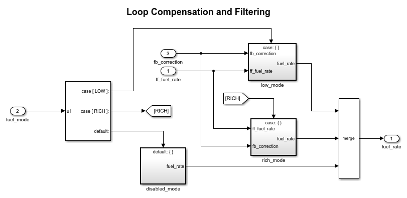
Figure 10: Switchable compensation subsystem

Results and Conclusions

Simulation results are shown in Figure 11 and Figure 12. The simulation is run with a throttle input that ramps from 10 to 20 degrees over a period of two seconds, then goes back to 10 degrees over the next two seconds. This cycle repeats continuously while the engine is held at a constant speed so that the user can experiment with different fault conditions and failure modes. Click on a sensor fault switch in the dashboard subsystem to simulate the failure of the associated sensor. Repeat this operation to slide the switch back for normal operation.

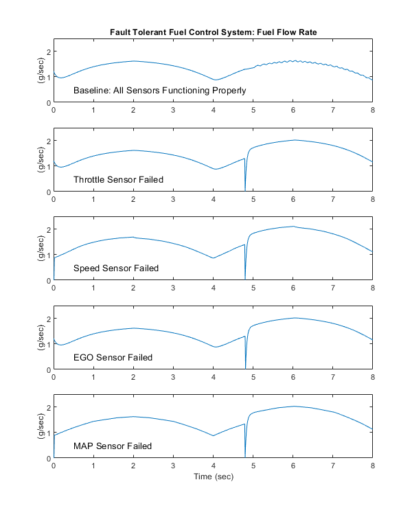
Figure 11: Comparing the fuel flow rate for different sensor failures

Figure 11 compares the fuel flow rate under fault-free conditions (baseline) with the rate applied in the presence of a single failure in each sensor individually. In each case note the nonlinear relationship between fuel flow and the triangular throttle command (shown in Figure 13). In the baseline case, the fuel rate is regulated tightly, exhibiting a small ripple due to the switching nature of the EGO sensor's input circuitry. In the other four cases the system operates open loop. The control strategy is proven effective in maintaining the correct fuel profile in the single-failure mode. In each of the fault conditions, the fuel rate is essentially 125% of the baseline flow, fulfilling the design objective of 80% rich.

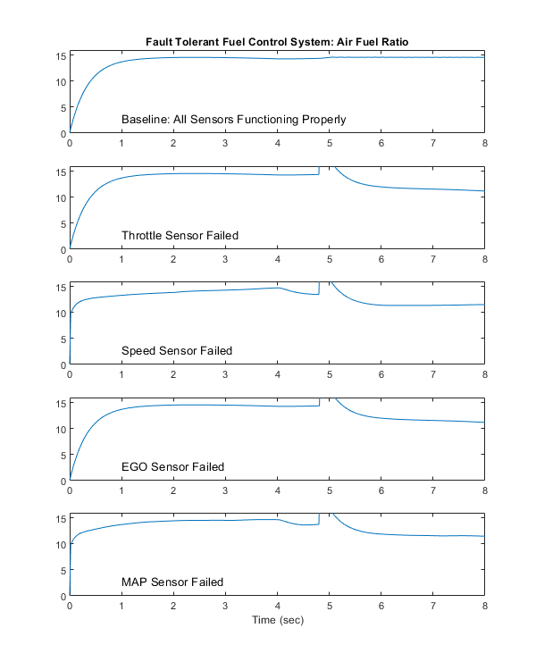
Figure 12: Comparing the air-fuel ratio for different sensor failures

Figure 12 plots the corresponding air/fuel ratio for each case. The baseline plot shows the effects of closed-loop operation. The mixture ratio is regulated very tightly to the stoichiometric objective of 14.6. The rich mixture ratio is shown in the bottom four plots of Figure 12. Although they are not tightly regulated, as in the closed-loop case, they approximate the objective of air/fuel (0.8*14.6=11.7).

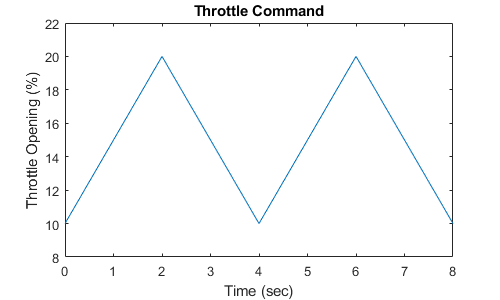
Figure 13: Throttle command

The transient behavior of the system is shown in Figure 14. With a constant 12 degree throttle angle and the system in steady-state, a throttle failure is introduced at t = 2 and corrected at t = 5. At the onset of the failure, the fuel rate increases immediately. The effects are seen at the exhaust as the rich ratio propagates through the system. The steady-state condition is then quickly recovered when closed-loop operation is restored.

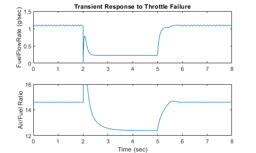
Figure 14: Transient response to fault detection

Remarks

If you enable animation in the Stateflow debugger, the state transitions are highlighted in the Stateflow diagram (see Figure 4) as the various states are activated. The sequence of activation is indicated by changing colors. This closely coupled synergy between Stateflow and Simulink fosters the modeling and development of complete control systems.