Workflow for Expected Shortfall (ES) Backtesting by Du and Escanciano
This example shows the workflow for using the Du-Escanciano (DE) expected shortfall (ES) backtests and demonstrates a fixed test window for a single DE model with multiple VaR levels.
Load Data
The data in the ESBacktestDistributionData.mat file has returns, VaR and ES data, and distribution information for three models: normal, and t with 5 degrees of freedom and t with 10 degrees of freedom. The data spans multiple years from January 1996 to July 2003 and includes a total of 1966 observations.
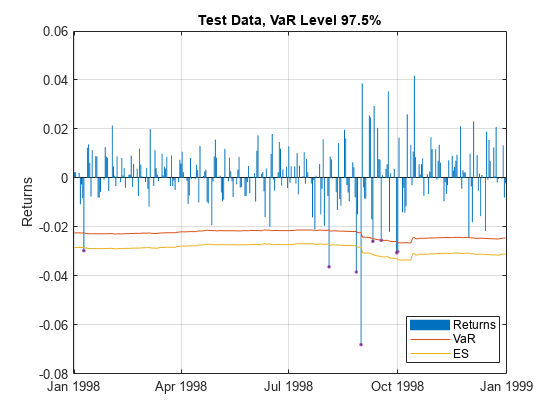
This example uses a t distribution with 10 degrees of freedom and focuses on one year of data to show the difference between the critical value methods for large-sample approximation and simulation supported by the esbacktestbyde class.
load ESBacktestDistributionData.mat

TargetYear = 1998; % Change to test other calendar years
Ind = year(Dates)==TargetYear;
Dates = Dates(Ind);
Returns = Returns(Ind);
VaR = T10VaR(Ind,:);
ES = T10ES(Ind,:);
Mu = 0; % Always 0 in this data set
Sigma = T10Scale(Ind);
Plot Data
Plot the data for a VaR level of 0.975.
% Plot data
TargetVaRLevel = 0.975;
VaRInd = VaRLevel==TargetVaRLevel;

FailureInd = Returns<-VaR(:,VaRInd);

bar(Dates,Returns)
hold on
plot(Dates,-VaR(:,VaRInd),Dates,-ES(:,VaRInd))
plot(Dates(FailureInd),Returns(FailureInd),'.')
hold off
legend('Returns','VaR','ES','Location','best')
title(['Test Data, VaR Level ' num2str(TargetVaRLevel*100) '%'])
ylabel('Returns')
grid on

Create an esbacktestbyde Object
Create an esbacktestbyde object to run the DE tests. Note that VaR and ES data are not required inputs because the DE tests work on "mapped returns" or "ranks" and perform mapping by using the distribution information. However, for convenience, the esbacktestbyde object computes the VaR and ES data internally using the distribution information and stores the data in the VaRData and ESData properties of the esbacktestbyde object. The VaR and ES data is used only to estimate the severity ratios reported by the summary function and are not used for any of the DE tests.
By default, when you create a esbacktestbyde object, a simulation runs and large-sample and simulation-based critical values are available immediately. Although the simulation processing is efficient, if you verify that large-sample approximation is appropriate for the sample size and VaR level under consideration, you can turn the simulation off to increase processing speed. To turn off the simulation, when using esbacktestbyde to create an esbacktestbtde object, set the name-value pair argument 'Simulate' to false.
rng('default'); % For reproducibility
tic;
ebtde = esbacktestbyde(Returns,"t",...
'DegreesOfFreedom',10,...
'Location',Mu,...
'Scale',Sigma,...
'VaRLevel',VaRLevel,...
'PortfolioID',"S&P",...
'VaRID',"t(10)");
toc;
Elapsed time is 0.146348 seconds.
disp(ebtde)
  esbacktestbyde with properties:

    PortfolioData: [261x1 double]
          VaRData: [261x3 double]
           ESData: [261x3 double]
     Distribution: [1x1 struct]
      PortfolioID: "S&P"
            VaRID: ["t(10)"    "t(10)"    "t(10)"]
         VaRLevel: [0.9500 0.9750 0.9900]
disp(ebtde.Distribution)
                Name: "t"
    DegreesOfFreedom: 10
            Location: 0
               Scale: [261x1 double]
Summary Statistics
Use summary to return a basic expected shortfall (ES) report on failures and severity. This is the same summary output as the other ES backtesting classes esbacktest and esbacktestbysim. When the esbacktestbyde object is created, the VaR and ES data are computed using the distribution information. This information is stored in the VaRData and ESData properties. The summary function uses the VaRData and ESData properties to compute the observed severity ratio.
disp(summary(ebtde))
    PortfolioID     VaRID     VaRLevel    ObservedLevel    ExpectedSeverity    ObservedSeverity    Observations    Failures    Expected    Ratio     Missing
    ___________    _______    ________    _____________    ________________    ________________    ____________    ________    ________    ______    _______

       "S&P"       "t(10)"      0.95         0.94253            1.3288              1.5295             261            15        13.05      1.1494       0
       "S&P"       "t(10)"     0.975         0.96935            1.2652              1.5269             261             8        6.525      1.2261       0
       "S&P"       "t(10)"      0.99         0.98467            1.2169              1.5786             261             4         2.61      1.5326       0
Run Tests
Use runtests to run all expected shortfall (ES) backtests for esbacktestbyde object. The default critical value method is 'large-sample' or asymptotic approximation.
disp(runtests(ebtde))
    PortfolioID     VaRID     VaRLevel    ConditionalDE    UnconditionalDE
    ___________    _______    ________    _____________    _______________

       "S&P"       "t(10)"      0.95         accept            accept
       "S&P"       "t(10)"     0.975         accept            accept
       "S&P"       "t(10)"      0.99         accept            accept
Run the tests with 'simulation' or finite-sample critical values.
disp(runtests(ebtde,'CriticalValueMethod','simulation'))
    PortfolioID     VaRID     VaRLevel    ConditionalDE    UnconditionalDE
    ___________    _______    ________    _____________    _______________

       "S&P"       "t(10)"      0.95         accept            accept
       "S&P"       "t(10)"     0.975         accept            accept
       "S&P"       "t(10)"      0.99         accept            accept
The runtests function accepts the name-value pair argument 'ShowDetails' which includes extra columns in the output. Specifically, this output includes the critical value method used, number of lags, and test confidence level.
disp(runtests(ebtde,'CriticalValueMethod','simulation','ShowDetails',true))
    PortfolioID     VaRID     VaRLevel    ConditionalDE    UnconditionalDE    CriticalValueMethod    NumLags    TestLevel
    ___________    _______    ________    _____________    _______________    ___________________    _______    _________

       "S&P"       "t(10)"      0.95         accept            accept            "simulation"           1         0.95
       "S&P"       "t(10)"     0.975         accept            accept            "simulation"           1         0.95
       "S&P"       "t(10)"      0.99         accept            accept            "simulation"           1         0.95
Unconditional DE Test Details
The unconditional DE test assesses the severity of the violations based on an evaluation of the observed average tail loss and determines whether the severity is consistent with the model assumptions. All the tests supported in the related classes esbacktest and esbacktestbysim are also severity tests.
To view the unconditional DE test details, use the unconditionalDE function. By default, this function uses the 'large-sample' critical value method.
disp(unconditionalDE(ebtde))
    PortfolioID     VaRID     VaRLevel    UnconditionalDE     PValue     TestStatistic     LowerCI     UpperCI     Observations    CriticalValueMethod    MeanLS      StdLS      Scenarios    TestLevel
    ___________    _______    ________    _______________    ________    _____________    _________    ________    ____________    ___________________    ______    _________    _________    _________

       "S&P"       "t(10)"      0.95          accept          0.31715      0.032842       0.0096343    0.040366        261           "large-sample"        0.025    0.0078398       NaN         0.95
       "S&P"       "t(10)"     0.975          accept          0.32497      0.018009       0.0015295    0.023471        261           "large-sample"       0.0125    0.0055973       NaN         0.95
       "S&P"       "t(10)"      0.99          accept         0.076391      0.011309               0    0.011978        261           "large-sample"        0.005    0.0035603       NaN         0.95
To compare the results of 'large-sample' to simulation-based critical values, use the name-value pair argument 'CriticalValueMethod'. In this example, the results of both critical value methods, including the confidence interval and the p-values, look similar.
disp(unconditionalDE(ebtde,'CriticalValueMethod','simulation'))
    PortfolioID     VaRID     VaRLevel    UnconditionalDE    PValue    TestStatistic     LowerCI     UpperCI     Observations    CriticalValueMethod    MeanLS    StdLS    Scenarios    TestLevel
    ___________    _______    ________    _______________    ______    _____________    _________    ________    ____________    ___________________    ______    _____    _________    _________

       "S&P"       "t(10)"      0.95          accept         0.326       0.032842        0.010859    0.041709        261            "simulation"         NaN       NaN       1000         0.95
       "S&P"       "t(10)"     0.975          accept         0.336       0.018009       0.0032446    0.024657        261            "simulation"         NaN       NaN       1000         0.95
       "S&P"       "t(10)"      0.99          accept         0.126       0.011309               0    0.013311        261            "simulation"         NaN       NaN       1000         0.95
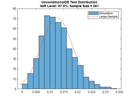
You can visualize the 'simulation' and 'large-sample' distributions to assess whether the 'large-sample' approximation is accurate enough for the sample size and VaR level under consideration. The unconditionalDE function returns the 'simulated' test statistics as an optional output.
In this example, higher VaR levels cause a noticeable mismatch between the 'large-sample' and 'simulation' distributions. However, the confidence intervals and p-values are comparable.
% Choose VaR level
TargetVaRLevel = 0.975;
VaRInd = VaRLevel==TargetVaRLevel;

[~,s] = unconditionalDE(ebtde,'CriticalValueMethod','simulation');
histogram(s(VaRInd,:),'Normalization',"pdf")
hold on
t = unconditionalDE(ebtde,'CriticalValueMethod','large-sample');
Mu = t.MeanLS(VaRInd);
Sigma = t.StdLS(VaRInd);
MinValPlot = min(s(VaRInd,:))-0.001;
MaxValPlot = max(s(VaRInd,:))+0.001;
xLS = linspace(MinValPlot,MaxValPlot,101);
pdfLS = normpdf(xLS,Mu,Sigma);
plot(xLS,pdfLS)
hold off
legend({'Simulation','Large-Sample'})
Title = sprintf('UnconditionalDE Test Distribution\nVaR Level: %g%%, Sample Size = %d',VaRLevel(VaRInd)*100,t.Observations(VaRInd));
title(Title)

Conditional DE Test Details
The conditional DE test assesses whether there is evidence of autocorrelation in the tail losses.
Although the names are similar, the conditional DE test and the conditional test supported in esbacktestbysim are qualitatively different tests. The conditional Acerbi-Szekely test supported in esbacktestbysim tests the severity of the ES, conditional on whether the model passes a VaR test. The Acerbi-Szekely conditional test is a severity test, comparable to the tests supported in esbacktest, esbacktestbysim, and the unconditionalDE test.
However, the conditional DE test in esbacktestbyde is a test for independence across time periods.
To see the details of the conditional DE test results, use the conditionalDE function. By default, this function uses the 'large-sample' critical value method and tests for one lag (correlation with the previous time period).
disp(conditionalDE(ebtde))
    PortfolioID     VaRID     VaRLevel    ConditionalDE    PValue     TestStatistic    CriticalValue    AutoCorrelation    Observations    CriticalValueMethod    NumLags    Scenarios    TestLevel
    ___________    _______    ________    _____________    _______    _____________    _____________    _______________    ____________    ___________________    _______    _________    _________

       "S&P"       "t(10)"      0.95         accept        0.45361        0.5616          3.8415            0.046387           261           "large-sample"          1          NaN         0.95
       "S&P"       "t(10)"     0.975         accept        0.54189       0.37205          3.8415            0.037755           261           "large-sample"          1          NaN         0.95
       "S&P"       "t(10)"      0.99         accept        0.87949      0.022989          3.8415          -0.0093851           261           "large-sample"          1          NaN         0.95
The results of the 'large-sample' critical value method, particularly the simulation critical values and p-values, differ substantially from the results of the 'simulation' critical value method.
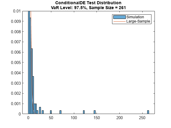
The critical value is similar for a 95% VaR level, but the simulation-based critical value is much larger for higher VaR levels, especially for a 99% VaR. The autocorrelation is 1 for any sample without VaR failures. Therefore, the test statistic equals the number of observations for any scenario without VaR failures. For a 99% VaR level, scenarios without VaR failures are like; consequently, there is a mass point at the number of observations which appears as a long, heavy tail in the simulated distribution of the test statistic.
disp(conditionalDE(ebtde,'CriticalValueMethod','simulation'))
    PortfolioID     VaRID     VaRLevel    ConditionalDE    PValue    TestStatistic    CriticalValue    AutoCorrelation    Observations    CriticalValueMethod    NumLags    Scenarios    TestLevel
    ___________    _______    ________    _____________    ______    _____________    _____________    _______________    ____________    ___________________    _______    _________    _________

       "S&P"       "t(10)"      0.95         accept        0.257         0.5616          3.6876            0.046387           261            "simulation"           1         1000         0.95
       "S&P"       "t(10)"     0.975         accept        0.141        0.37205          5.3504            0.037755           261            "simulation"           1         1000         0.95
       "S&P"       "t(10)"      0.99         accept        0.502       0.022989             261          -0.0093851           261            "simulation"           1         1000         0.95
You can visually compare the 'large-sample' and 'simulation' distributions. The conditionalDE function also returns the simulated test statistics as an optional output.
Notice that the tail of the distribution gets heavier as the VaR level increases.
% Choose VaR level
TargetVaRLevel = 0.975;
VaRInd = VaRLevel==TargetVaRLevel;

[t,s] = conditionalDE(ebtde,'CriticalValueMethod','simulation');
xLS = 0:0.01:20;
pdfLS = chi2pdf(xLS,t.NumLags(1));
histogram(s(VaRInd,:),'Normalization',"pdf")
hold on
plot(xLS,pdfLS)
hold off
ylim([0 0.01])
legend({'Simulation','Large-Sample'})
Title = sprintf('ConditionalDE Test Distribution\nVaR Level: %g%%, Sample Size = %d',VaRLevel(VaRInd)*100,t.Observations(VaRInd));
title(Title)

Because the conditional DE test is based on autocorrelations, you can run the test for differing numbers of lags.
Run the conditional DE test for 2 lags. At a VaR level of 99%, the 'large-sample' critical value method rejects the model but the 'simulation' critical value method does not reject the model, with a p-value close to 10%. This shows that the 'simulation' distribution and the 'large-sample' approximation can lead to different results, depending on the sample size and VaR level.
disp(conditionalDE(ebtde,'NumLags',2,'CriticalValueMethod','large-sample'))
    PortfolioID     VaRID     VaRLevel    ConditionalDE      PValue      TestStatistic    CriticalValue    AutoCorrelation    Observations    CriticalValueMethod    NumLags    Scenarios    TestLevel
    ___________    _______    ________    _____________    __________    _____________    _____________    _______________    ____________    ___________________    _______    _________    _________

       "S&P"       "t(10)"      0.95         reject          0.015812        8.294           5.9915            0.17212            261           "large-sample"          2          NaN         0.95
       "S&P"       "t(10)"     0.975         reject        0.00045758       15.379           5.9915            0.23979            261           "large-sample"          2          NaN         0.95
       "S&P"       "t(10)"      0.99         reject        2.5771e-07       30.343           5.9915            0.34083            261           "large-sample"          2          NaN         0.95
disp(conditionalDE(ebtde,'NumLags',2,'CriticalValueMethod','simulation'))
    PortfolioID     VaRID     VaRLevel    ConditionalDE    PValue    TestStatistic    CriticalValue    AutoCorrelation    Observations    CriticalValueMethod    NumLags    Scenarios    TestLevel
    ___________    _______    ________    _____________    ______    _____________    _____________    _______________    ____________    ___________________    _______    _________    _________

       "S&P"       "t(10)"      0.95         reject         0.03         8.294           6.1397            0.17212            261            "simulation"           2         1000         0.95
       "S&P"       "t(10)"     0.975         reject        0.019        15.379           9.3364            0.23979            261            "simulation"           2         1000         0.95
       "S&P"       "t(10)"      0.99         accept        0.098        30.343              522            0.34083            261            "simulation"           2         1000         0.95
Running a New Simulation with simulate
If a p-value is near a rejection boundary, you can run a new simulation to request more scenarios to reduce a simulation error.
You can also run a new simulation to request a higher number of lags. By default, creating an esbacktestbyde object causes the simulation to run so that the simulation test results are available immediately. However, to avoid extra storage, only 5 lags are simulated. If you request more than 5 lags with the simulate function, the conditionalDE test function displays the following message:
No simulation results available for the number of lags requested. Call 'simulate' with the desired number of lags.
You first need to run a new simulation using esbacktestbyde and specify the number of lags to use for that simulation. Displaying the size of the esbacktestbyde object before and after the new simulation illustrates how simulating with more lags increases the amount of data stored in the esbacktestbyde object, as more simulated test statistics are stored with more lags.
% See bytes before new simulation, 5 lags stored
whos ebtde
  Name       Size             Bytes  Class             Attributes

  ebtde      1x1             164883  esbacktestbyde
% Simulate 6 lags
rng('default'); % for reproducibility
ebtde = simulate(ebtde,'NumLags',6);

% See bytes after new simulation, 6 lags stored
whos ebtde
  Name       Size             Bytes  Class             Attributes

  ebtde      1x1             188891  esbacktestbyde
After you run a new simulation with esbacktestbyde that increases the number of lags to 6, the test results for conditionalDE are available for the 'simulation' method using 6 lags.
disp(conditionalDE(ebtde,'NumLags',6,'CriticalValueMethod','simulation'))
    PortfolioID     VaRID     VaRLevel    ConditionalDE    PValue    TestStatistic    CriticalValue    AutoCorrelation    Observations    CriticalValueMethod    NumLags    Scenarios    TestLevel
    ___________    _______    ________    _____________    ______    _____________    _____________    _______________    ____________    ___________________    _______    _________    _________

       "S&P"       "t(10)"      0.95         accept        0.136        9.5173           16.412           -0.022881           261            "simulation"           6         1000         0.95
       "S&P"       "t(10)"     0.975         accept        0.086        15.854           21.299           -0.021864           261            "simulation"           6         1000         0.95
       "S&P"       "t(10)"      0.99         accept        0.128        30.438             1566          -0.0096211           261            "simulation"           6         1000         0.95
Alternatively, the conditionalDE test results are always available for the 'large-sample' method for any number of lags.
disp(conditionalDE(ebtde,'NumLags',10,'CriticalValueMethod','large-sample'))
    PortfolioID     VaRID     VaRLevel    ConditionalDE      PValue      TestStatistic    CriticalValue    AutoCorrelation    Observations    CriticalValueMethod    NumLags    Scenarios    TestLevel
    ___________    _______    ________    _____________    __________    _____________    _____________    _______________    ____________    ___________________    _______    _________    _________

       "S&P"       "t(10)"      0.95         reject          0.018711       21.361           18.307             0.15415           261           "large-sample"         10          NaN         0.95
       "S&P"       "t(10)"     0.975         accept          0.088587       16.406           18.307            0.027955           261           "large-sample"         10          NaN         0.95
       "S&P"       "t(10)"      0.99         reject        0.00070234       30.526           18.307          -0.0092432           261           "large-sample"         10          NaN         0.95
See Also
esbacktestbyde | esbacktest | esbacktestbysim | varbacktest
Related Topics
- VaR Backtesting Workflow
- Value-at-Risk Estimation and Backtesting
- Expected Shortfall (ES) Backtesting Workflow with No Model Distribution Information
- Expected Shortfall (ES) Backtesting Workflow Using Simulation
- Expected Shortfall Estimation and Backtesting
- Rolling Windows and Multiple Models for Expected Shortfall (ES) Backtesting by Du and Escanciano
