bat365 Homepage

Expected Shortfall Estimation and Backtesting

This example shows how to perform estimation and backtesting of Expected Shortfall models.

Value-at-Risk (VaR) and Expected Shortfall (ES) must be estimated together because the ES estimate depends on the VaR estimate. Using historical data, this example estimates VaR and ES over a test window, using historical and parametric VaR approaches. The parametric VaR is calculated under the assumption of normal and t distributions.

This example runs the ES back tests supported in the esbacktest, esbacktestbysim, and esbacktestbyde functionality to assess the performance of the ES models in the test window.

The esbacktest object does not require any distribution information. Like the varbacktest object, the esbacktest object only takes test data as input. The inputs to esbacktest include portfolio data, VaR data and corresponding VaR level, and also the ES data, since this is what is back tested. Like varbacktest, esbacktest runs tests for a single portfolio, but can back test multiple models and multiple VaR levels at once. The esbacktest object uses precomputed tables of critical values to determine if the models should be rejected. These table-based tests can be applied as approximate tests for any VaR model. In this example, they are applied to back test historical and parametric VaR models. They could be used for other VaR approaches such as Monte-Carlo or Extreme-Value models.

In contrast, the esbacktestbysim and esbacktestbyde objects require the distribution information, namely, the distribution name (normal or t) and the distribution parameters for each day in the test window. esbacktestbysim and esbacktestbyde can only back test one model at a time because they are linked to a particular distribution, although you can still back test multiple VaR levels at once. The esbacktestbysim object implements simulation-based tests and it uses the provided distribution information to run simulations to determine critical values. The esbacktestbyde object implements tests where the critical values are derived from either a large-sample approximation or a simulation (finite sample). The conditionalDE test in the esbacktestbyde object tests for independence over time, to assess if there is evidence of autocorrelation in the series of tail losses. All other tests are severity tests to assess if the magnitude of the tail losses is consistent with the model predictions. Both the esbacktestbysim and esbacktestbyde objects support normal and t distributions. These tests can be used for any model where the underlying distribution of portfolio outcomes is normal or t, such as exponentially weighted moving average (EWMA), delta-gamma, or generalized autoregressive conditional heteroskedasticity (GARCH) models.

For additional information on the ES backtesting methodology, see esbacktest, esbacktestbysim, and esbacktestbyde, also see [1], [2], [3] and [5] in the References.

Estimate VaR and ES

The data set used in this example contains historical data for the S&P index spanning approximately 10 years, from the middle of 1993 through the middle of 2003. The estimation window size is defined as 250 days, so that a full year of data is used to estimate both the historical VaR, and the volatility. The test window in this example runs from the beginning of 1995 through the end of 2002.

Throughout this example, a VaR confidence level of 97.5% is used, as required by the Fundamental Review of the Trading Book (FRTB) regulation; see [4].

load VaRExampleData.mat
Returns = tick2ret(sp);
DateReturns = dates(2:end);
SampleSize = length(Returns);

TestWindowStart = find(year(DateReturns)==1995,1);
TestWindowEnd = find(year(DateReturns)==2002,1,'last');
TestWindow = TestWindowStart:TestWindowEnd;
EstimationWindowSize = 250;

DatesTest = DateReturns(TestWindow);
ReturnsTest = Returns(TestWindow);

VaRLevel = 0.975;

The historical VaR is a non-parametric approach to estimate the VaR and ES from historical data over an estimation window. The VaR is a percentile, and there are alternative ways to estimate the percentile of a distribution based on a finite sample. One common approach is to use the prctile function. An alternative approach is to sort the data and determine a cut point based on the sample size and VaR confidence level. Similarly, there are alternative approaches to estimate the ES based on a finite sample.

The hHistoricalVaRES local function on the bottom of this example uses a finite-sample approach for the estimation of VaR and ES following the methodology described in [7]. In a finite sample, the number of observations below the VaR may not match the total tail probability corresponding to the VaR level. For example, for 100 observations and a VaR level of 97.5%, the tail observations are 2, which is 2% of the sample, however the desired tail probability is 2.5%. It could be even worse for samples with repeated observed values, for example, if the second and third sorted values were the same, both equal to the VaR, then only the smallest observed value in the sample would have a value less than the VaR, and that is 1% of the sample, not the desired 2.5%. The method implemented in hHistoricalVaRES makes a correction so that the tail probability is always consistent with the VaR level; see [7] for details.

VaR_Hist = zeros(length(TestWindow),1);
ES_Hist = zeros(length(TestWindow),1);

for t = TestWindow
   
   i = t - TestWindowStart + 1;
   EstimationWindow = t-EstimationWindowSize:t-1;
   
   [VaR_Hist(i),ES_Hist(i)] = hHistoricalVaRES(Returns(EstimationWindow),VaRLevel);
   
end

The following plot shows the daily returns, and the VaR and ES estimated with the historical method.

figure;
plot(DatesTest,ReturnsTest,DatesTest,-VaR_Hist,DatesTest,-ES_Hist)
legend('Returns','VaR','ES','Location','southeast')
title('Historical VaR and ES')
grid on

Figure contains an axes object. The axes object with title Historical VaR and ES contains 3 objects of type line. These objects represent Returns, VaR, ES.

For the parametric models, the volatility of the returns must be computed. Given the volatility, the VaR, and ES can be computed analytically.

A zero mean is assumed in this example, but can be estimated in a similar way.

For the normal distribution, the estimated volatility is used directly to get the VaR and ES. For the t location-scale distribution, the scale parameter is computed from the estimated volatility and the degrees of freedom.

The hNormalVaRES and hTVaRES local functions take as inputs the distribution parameters (which can be passed as arrays), and return the VaR and ES. These local functions use the analytical expressions for VaR and ES for normal and t location-scale distributions, respectively; see [6] for details.

% Estimate volatility over the test window
Volatility = zeros(length(TestWindow),1);

for t = TestWindow
   
   i = t - TestWindowStart + 1;
   EstimationWindow = t-EstimationWindowSize:t-1;
   
   Volatility(i) = std(Returns(EstimationWindow));
   
end

% Mu=0 in this example
Mu = 0;

% Sigma (standard deviation parameter) for normal distribution = Volatility
SigmaNormal = Volatility;
% Sigma (scale parameter) for t distribution = Volatility * sqrt((DoF-2)/DoF)
SigmaT10 = Volatility*sqrt((10-2)/10);
SigmaT5 = Volatility*sqrt((5-2)/5);

% Estimate VaR and ES, normal
[VaR_Normal,ES_Normal] = hNormalVaRES(Mu,SigmaNormal,VaRLevel);
% Estimate VaR and ES, t with 10 and 5 degrees of freedom
[VaR_T10,ES_T10] = hTVaRES(10,Mu,SigmaT10,VaRLevel);
[VaR_T5,ES_T5] = hTVaRES(5,Mu,SigmaT5,VaRLevel);

The following plot shows the daily returns, and the VaR and ES estimated with the normal method.

figure;
plot(DatesTest,ReturnsTest,DatesTest,-VaR_Normal,DatesTest,-ES_Normal)
legend('Returns','VaR','ES','Location','southeast')
title('Normal VaR and ES')
grid on

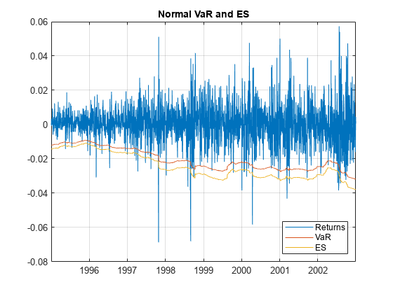
Figure contains an axes object. The axes object with title Normal VaR and ES contains 3 objects of type line. These objects represent Returns, VaR, ES.

For the parametric approach, the same steps can be used to estimate the VaR and ES for alternative approaches, such as EWMA, delta-gamma approximations, and GARCH models. In all these parametric approaches, a volatility is estimated every day, either from an EWMA update, from a delta-gamma approximation, or as the conditional volatility of a GARCH model. The volatility can then be used as above to get the VaR and ES estimates for either normal or t location-scale distributions.

ES Backtest Without Distribution Information

The esbacktest object offers two back tests for ES models. Both tests use the unconditional test statistic proposed by Acerbi and Szekely in [1], given by

$Z_{uncond} = \frac{1}{{Np}_{VaR}} \sum_{t = 1}^{N} \frac{X_{t} I_{t}}{{ES}_{t}} + 1$

where

$N$ is the number of time periods in the test window.
$X_{t}$ is the portfolio outcome, that is, the portfolio return or portfolio profit and loss for period t.
$p_{VaR}$ is the probability of VaR failure defined as 1-VaR level.
${ES}_{t}$ is the estimated expected shortfall for period t.
$I_{t}$ is the VaR failure indicator on period t with a value of 1 if $X_{t} < {- VaR}_{t}$ , and 0 otherwise.

The expected value for this test statistic is 0, and it is negative when there is evidence of risk underestimation. To determine how negative it should be to reject the model, critical values are needed, and to determine critical values, distributional assumptions are needed for the portfolio outcomes $X_{t}$ .

The unconditional test statistic turns out to be stable across a range of distributional assumptions for $X_{t}$ , from thin-tailed distributions such as normal, to heavy-tailed distributions such as t with low degrees of freedom (high single digits). Only the most heavy-tailed t distributions (low single digits) lead to more noticeable differences in the critical values. See [1] for details.

The esbacktest object takes advantage of the stability of the critical values of the unconditional test statistic and uses tables of precomputed critical values to run ES back tests. esbacktest has two sets of critical-value tables. The first set of critical values assumes that the portfolio outcomes $X_{t}$ follow a standard normal distribution; this is the unconditionalNormal test. The second set of critical values uses the heaviest possible tails, it assumes that the portfolio outcomes $X_{t}$ follow a t distribution with 3 degrees of freedom; this is the unconditionalT test.

The unconditional test statistic is sensitive to both the severity of the VaR failures relative to the ES estimate, and also to the number of VaR failures (how many times the VaR is violated). Therefore, a single but very large VaR failure relative to the ES (or only very few large losses) may cause the rejection of a model in a particular time window. A large loss on a day when the ES estimate is also large may not impact the test results as much as a large loss when the ES is smaller. And a model can also be rejected in periods with many VaR failures, even if all the VaR violations are relatively small and only slightly higher than the VaR. Both situations are illustrated in this example.

The esbacktest object takes as input the test data, but no distribution information is provided to esbacktest. Optionally, you can specify ID's for the portfolio, and for each of the VaR and ES models being backtested. Although the model ID's in this example do have distribution references (for example, "normal" or "t 10"), these are only labels used for reporting purposes. The tests do not use the fact that the first model is a historical VaR method, or that the other models are alternative parametric VaR models. The distribution parameters used to estimate the VaR and ES in the previous section are not passed to esbacktest, and are not used in any way in this section. These parameters, however, must be provided for the simulation-based tests supported in the esbacktestbysim object discussed in the Simulation-Based Tests section, and for the tests supported in the esbacktestbyde object discussed in the Large-Sample and Simulation Tests section.

ebt = esbacktest(ReturnsTest,[VaR_Hist VaR_Normal VaR_T10 VaR_T5],...
   [ES_Hist ES_Normal ES_T10 ES_T5],'PortfolioID',"S&P, 1995-2002",...
   'VaRID',["Historical" "Normal","T 10","T 5"],'VaRLevel',VaRLevel);
disp(ebt)

  esbacktest with properties:

    PortfolioData: [2087x1 double]
          VaRData: [2087x4 double]
           ESData: [2087x4 double]
      PortfolioID: "S&P, 1995-2002"
            VaRID: ["Historical"    "Normal"    "T 10"    "T 5"]
         VaRLevel: [0.9750 0.9750 0.9750 0.9750]

Start the analysis by running the summary function.

s = summary(ebt);
disp(s)

      PortfolioID          VaRID        VaRLevel    ObservedLevel    ExpectedSeverity    ObservedSeverity    Observations    Failures    Expected    Ratio     Missing
    ________________    ____________    ________    _____________    ________________    ________________    ____________    ________    ________    ______    _______

    "S&P, 1995-2002"    "Historical"     0.975         0.96694            1.3711              1.4039             2087           69        52.175     1.3225       0   
    "S&P, 1995-2002"    "Normal"         0.975         0.97077            1.1928               1.416             2087           61        52.175     1.1691       0   
    "S&P, 1995-2002"    "T 10"           0.975         0.97173            1.2652              1.4063             2087           59        52.175     1.1308       0   
    "S&P, 1995-2002"    "T 5"            0.975         0.97173              1.37              1.4075             2087           59        52.175     1.1308       0

The ObservedSeverity column shows the average ratio of loss to VaR on periods when the VaR was violated. The ExpectedSeverity column uses the average ratio of ES to VaR for the VaR violation periods. For the "Historical" and "T 5" models, the observed and expected severities are comparable. However, for the "Historical" method, the observed number of failures (Failures column) is considerably higher than the expected number of failures (Expected column), about 32% higher (see the Ratio column). Both the "Normal" and the "T 10" models have observed severities much higher than the expected severities.

figure;

subplot(2,1,1)
bar(categorical(s.VaRID),[s.ExpectedSeverity,s.ObservedSeverity])
ylim([1 1.5])
legend('Expected','Observed','Location','southeast')
title('Average Severity Ratio')

subplot(2,1,2)
bar(categorical(s.VaRID),[s.Expected,s.Failures])
ylim([40 70])
legend('Expected','Observed','Location','southeast')
title('Number of VaR Failures')

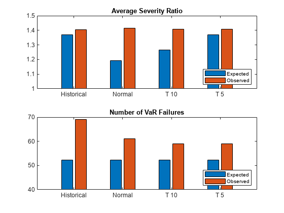
Figure contains 2 axes objects. Axes object 1 with title Average Severity Ratio contains 2 objects of type bar. These objects represent Expected, Observed. Axes object 2 with title Number of VaR Failures contains 2 objects of type bar. These objects represent Expected, Observed.

The runtests function runs all tests and reports only the accept or reject result. The unconditional normal test is more strict. For the 8-year test window here, two models fail both tests ("Historical" and "Normal"), one model fails the unconditional normal test, but passes the unconditional t test ("T 10"), and one model passes both tests ("T 5").

t = runtests(ebt);
disp(t)

      PortfolioID          VaRID        VaRLevel    UnconditionalNormal    UnconditionalT
    ________________    ____________    ________    ___________________    ______________

    "S&P, 1995-2002"    "Historical"     0.975            reject               reject    
    "S&P, 1995-2002"    "Normal"         0.975            reject               reject    
    "S&P, 1995-2002"    "T 10"           0.975            reject               accept    
    "S&P, 1995-2002"    "T 5"            0.975            accept               accept

Additional details on the tests can be obtained by calling the individual test functions. Here are the details for the unconditionalNormal test.

t = unconditionalNormal(ebt);
disp(t)

      PortfolioID          VaRID        VaRLevel    UnconditionalNormal     PValue      TestStatistic    CriticalValue    Observations    TestLevel
    ________________    ____________    ________    ___________________    _________    _____________    _____________    ____________    _________

    "S&P, 1995-2002"    "Historical"     0.975            reject           0.0047612      -0.37917         -0.23338           2087          0.95   
    "S&P, 1995-2002"    "Normal"         0.975            reject           0.0043287      -0.38798         -0.23338           2087          0.95   
    "S&P, 1995-2002"    "T 10"           0.975            reject            0.037528       -0.2569         -0.23338           2087          0.95   
    "S&P, 1995-2002"    "T 5"            0.975            accept             0.13069      -0.16179         -0.23338           2087          0.95

Here are the details for the unconditionalT test.

t = unconditionalT(ebt);
disp(t)

      PortfolioID          VaRID        VaRLevel    UnconditionalT     PValue     TestStatistic    CriticalValue    Observations    TestLevel
    ________________    ____________    ________    ______________    ________    _____________    _____________    ____________    _________

    "S&P, 1995-2002"    "Historical"     0.975          reject        0.017032      -0.37917         -0.27415           2087          0.95   
    "S&P, 1995-2002"    "Normal"         0.975          reject        0.015375      -0.38798         -0.27415           2087          0.95   
    "S&P, 1995-2002"    "T 10"           0.975          accept        0.062835       -0.2569         -0.27415           2087          0.95   
    "S&P, 1995-2002"    "T 5"            0.975          accept         0.16414      -0.16179         -0.27415           2087          0.95

Using the Tests for More Advanced Analyses

This section shows how to use the esbacktest object to run user-defined traffic-light tests, and also how to run tests over rolling test windows.

One way to define a traffic-light test is by combining the results from the unconditional normal and the unconditional t tests. Because the unconditional normal is more strict, one can define a traffic-light test with these levels:

Green: The model passes both the unconditional normal and unconditional t tests.
Yellow: The model fails the unconditional normal test, but passes the unconditional t test.
Red: The model is rejected by both the unconditional normal and unconditional t tests.

t = runtests(ebt);
TLValue = (t.UnconditionalNormal=='reject')+(t.UnconditionalT=='reject');
t.TrafficLight = categorical(TLValue,0:2,{'green','yellow','red'},'Ordinal',true);
disp(t)

      PortfolioID          VaRID        VaRLevel    UnconditionalNormal    UnconditionalT    TrafficLight
    ________________    ____________    ________    ___________________    ______________    ____________

    "S&P, 1995-2002"    "Historical"     0.975            reject               reject           red      
    "S&P, 1995-2002"    "Normal"         0.975            reject               reject           red      
    "S&P, 1995-2002"    "T 10"           0.975            reject               accept           yellow   
    "S&P, 1995-2002"    "T 5"            0.975            accept               accept           green

An alternative user-defined traffic-light test can use a single test, but at different test confidence levels:

Green: The result is to 'accept' with a test level of 95%.
Yellow: The result is to 'reject' at a 95% test level, but 'accept' at 99%.
Red: The result is 'reject' at 99% test level.

A similar test is proposed in [1] with a high test level of 99.99%.

t95 = runtests(ebt); % 95% is the default test level value
t99 = runtests(ebt,'TestLevel',0.99);
TLValue = (t95.UnconditionalNormal=='reject')+(t99.UnconditionalNormal=='reject');
tRolling = t95(:,1:3);
tRolling.UnconditionalNormal95 = t95.UnconditionalNormal;
tRolling.UnconditionalNormal99 = t99.UnconditionalNormal;
tRolling.TrafficLight = categorical(TLValue,0:2,{'green','yellow','red'},'Ordinal',true);
disp(tRolling)

      PortfolioID          VaRID        VaRLevel    UnconditionalNormal95    UnconditionalNormal99    TrafficLight
    ________________    ____________    ________    _____________________    _____________________    ____________

    "S&P, 1995-2002"    "Historical"     0.975             reject                   reject               red      
    "S&P, 1995-2002"    "Normal"         0.975             reject                   reject               red      
    "S&P, 1995-2002"    "T 10"           0.975             reject                   accept               yellow   
    "S&P, 1995-2002"    "T 5"            0.975             accept                   accept               green

The test results may be different over different test windows. Here, a one-year rolling window is used to run the ES back tests over the eight individual years spanned by the original test window. The first user-defined traffic-light described above is added to the test results table. The summary function is also called for each individual year to view the history of the severity and the number of VaR failures.

sRolling = table;
tRolling = table;
for Year = 1995:2002
   Ind = year(DatesTest)==Year;
   PortID = ['S&P, ' num2str(Year)];
   PortfolioData = ReturnsTest(Ind);
   VaRData = [VaR_Hist(Ind) VaR_Normal(Ind) VaR_T10(Ind) VaR_T5(Ind)];
   ESData = [ES_Hist(Ind) ES_Normal(Ind) ES_T10(Ind) ES_T5(Ind)];
   ebt = esbacktest(PortfolioData,VaRData,ESData,...
      'PortfolioID',PortID,'VaRID',["Historical" "Normal" "T 10" "T 5"],...
      'VaRLevel',VaRLevel);
   if Year == 1995
      sRolling = summary(ebt);
      tRolling = runtests(ebt);
   else
      sRolling = [sRolling;summary(ebt)]; %#ok<AGROW> 
      tRolling = [tRolling;runtests(ebt)]; %#ok<AGROW> 
   end
end

% Optional: Add the first user-defined traffic light test described above
TLValue = (tRolling.UnconditionalNormal=='reject')+(tRolling.UnconditionalT=='reject');
tRolling.TrafficLight = categorical(TLValue,0:2,{'green','yellow','red'},'Ordinal',true);

Display the results, one model at a time. The "T 5" model has the best performance in these tests (two "yellow"), and the "Normal" model the worst (three "red" and one "yellow").

disp(tRolling(tRolling.VaRID=="Historical",:))

    PortfolioID       VaRID        VaRLevel    UnconditionalNormal    UnconditionalT    TrafficLight
    ___________    ____________    ________    ___________________    ______________    ____________

    "S&P, 1995"    "Historical"     0.975            accept               accept           green    
    "S&P, 1996"    "Historical"     0.975            reject               accept           yellow   
    "S&P, 1997"    "Historical"     0.975            reject               reject           red      
    "S&P, 1998"    "Historical"     0.975            accept               accept           green    
    "S&P, 1999"    "Historical"     0.975            accept               accept           green    
    "S&P, 2000"    "Historical"     0.975            accept               accept           green    
    "S&P, 2001"    "Historical"     0.975            accept               accept           green    
    "S&P, 2002"    "Historical"     0.975            reject               reject           red

disp(tRolling(tRolling.VaRID=="Normal",:))

    PortfolioID     VaRID      VaRLevel    UnconditionalNormal    UnconditionalT    TrafficLight
    ___________    ________    ________    ___________________    ______________    ____________

    "S&P, 1995"    "Normal"     0.975            accept               accept           green    
    "S&P, 1996"    "Normal"     0.975            reject               reject           red      
    "S&P, 1997"    "Normal"     0.975            reject               reject           red      
    "S&P, 1998"    "Normal"     0.975            reject               accept           yellow   
    "S&P, 1999"    "Normal"     0.975            accept               accept           green    
    "S&P, 2000"    "Normal"     0.975            accept               accept           green    
    "S&P, 2001"    "Normal"     0.975            accept               accept           green    
    "S&P, 2002"    "Normal"     0.975            reject               reject           red

disp(tRolling(tRolling.VaRID=="T 10",:))

    PortfolioID    VaRID     VaRLevel    UnconditionalNormal    UnconditionalT    TrafficLight
    ___________    ______    ________    ___________________    ______________    ____________

    "S&P, 1995"    "T 10"     0.975            accept               accept           green    
    "S&P, 1996"    "T 10"     0.975            reject               reject           red      
    "S&P, 1997"    "T 10"     0.975            reject               accept           yellow   
    "S&P, 1998"    "T 10"     0.975            accept               accept           green    
    "S&P, 1999"    "T 10"     0.975            accept               accept           green    
    "S&P, 2000"    "T 10"     0.975            accept               accept           green    
    "S&P, 2001"    "T 10"     0.975            accept               accept           green    
    "S&P, 2002"    "T 10"     0.975            reject               reject           red

disp(tRolling(tRolling.VaRID=="T 5",:))

    PortfolioID    VaRID    VaRLevel    UnconditionalNormal    UnconditionalT    TrafficLight
    ___________    _____    ________    ___________________    ______________    ____________

    "S&P, 1995"    "T 5"     0.975            accept               accept           green    
    "S&P, 1996"    "T 5"     0.975            reject               accept           yellow   
    "S&P, 1997"    "T 5"     0.975            accept               accept           green    
    "S&P, 1998"    "T 5"     0.975            accept               accept           green    
    "S&P, 1999"    "T 5"     0.975            accept               accept           green    
    "S&P, 2000"    "T 5"     0.975            accept               accept           green    
    "S&P, 2001"    "T 5"     0.975            accept               accept           green    
    "S&P, 2002"    "T 5"     0.975            reject               accept           yellow

The year 2002 is an example of a year with relatively small severities, yet many VaR failures. All models perform poorly in 2002, even though the observed severities are low. However, the number of VaR failures for some models is more than twice the expected number of VaR failures.

disp(summary(ebt))

    PortfolioID       VaRID        VaRLevel    ObservedLevel    ExpectedSeverity    ObservedSeverity    Observations    Failures    Expected    Ratio     Missing
    ___________    ____________    ________    _____________    ________________    ________________    ____________    ________    ________    ______    _______

    "S&P, 2002"    "Historical"     0.975         0.94636            1.2022                 1.2             261            14        6.525      2.1456       0   
    "S&P, 2002"    "Normal"         0.975         0.94636            1.1928              1.2111             261            14        6.525      2.1456       0   
    "S&P, 2002"    "T 10"           0.975         0.95019            1.2652              1.2066             261            13        6.525      1.9923       0   
    "S&P, 2002"    "T 5"            0.975         0.95019              1.37              1.2077             261            13        6.525      1.9923       0

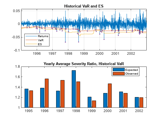
The following figure shows the data on the entire 8-year window, and severity ratio year by year (expected and observed) for the "Historical" model. The absolute size of the losses is not as important as the relative size compared to the ES (or equivalently, compared to the VaR). Both 1997 and 1998 have large losses, comparable in magnitude. However the expected severity in 1998 is much higher (larger ES estimates). Overall, the "Historical" method seems to do well with respect to severity ratios.

sH = sRolling(sRolling.VaRID=="Historical",:);

figure;

subplot(2,1,1)
FailureInd = ReturnsTest<-VaR_Hist;
plot(DatesTest,ReturnsTest,DatesTest,-VaR_Hist,DatesTest,-ES_Hist)
hold on
plot(DatesTest(FailureInd),ReturnsTest(FailureInd),'.')
hold off
legend('Returns','VaR','ES','Location','best')
title('Historical VaR and ES')
grid on

subplot(2,1,2)
bar(1995:2002,[sH.ExpectedSeverity,sH.ObservedSeverity])
ylim([1 1.8])
legend('Expected','Observed','Location','best')
title('Yearly Average Severity Ratio, Historical VaR')

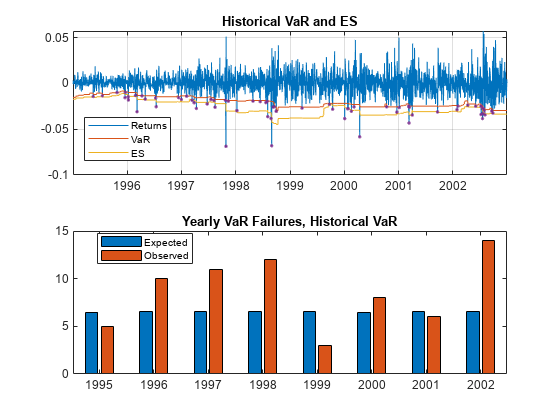
Figure contains 2 axes objects. Axes object 1 with title Historical VaR and ES contains 4 objects of type line. One or more of the lines displays its values using only markers These objects represent Returns, VaR, ES. Axes object 2 with title Yearly Average Severity Ratio, Historical VaR contains 2 objects of type bar. These objects represent Expected, Observed.

However, a similar visualization with the expected against observed number of VaR failures shows that the "Historical" method tends to get violated many more times than expected. For example, even though in 2002 the expected average severity ratio is very close to the observed one, the number of VaR failures was more than twice the expected number. This then leads to test failures for both the unconditional normal and unconditional t tests.

figure;

subplot(2,1,1)
plot(DatesTest,ReturnsTest,DatesTest,-VaR_Hist,DatesTest,-ES_Hist)
hold on
plot(DatesTest(FailureInd),ReturnsTest(FailureInd),'.')
hold off
legend('Returns','VaR','ES','Location','best')
title('Historical VaR and ES')
grid on

subplot(2,1,2)
bar(1995:2002,[sH.Expected,sH.Failures])
legend('Expected','Observed','Location','best')
title('Yearly VaR Failures, Historical VaR')

Figure contains 2 axes objects. Axes object 1 with title Historical VaR and ES contains 4 objects of type line. One or more of the lines displays its values using only markers These objects represent Returns, VaR, ES. Axes object 2 with title Yearly VaR Failures, Historical VaR contains 2 objects of type bar. These objects represent Expected, Observed.

Simulation-Based Tests

The esbacktestbysim object supports five simulation-based ES back tests. esbacktestbysim requires the distribution information for the portfolio outcomes, namely, the distribution name ("normal" or "t") and the distribution parameters for each day in the test window. esbacktestbysim uses the provided distribution information to run simulations to determine critical values. The tests supported in esbacktestbysim are conditional, unconditional, quantile, minBiasAbsolute, and minBiasRelative. These are implementations of the tests proposed by Acerbi and Szekely in [1], and [2], [3] for 2017 and 2019.

The esbacktestbysim object supports normal and t distributions. These tests can be used for any model where the underlying distribution of portfolio outcomes is normal or t, such as exponentially weighted moving average (EWMA), delta-gamma, or generalized autoregressive conditional heteroskedasticity (GARCH) models.

ES backtests are necessarily approximated in that they are sensitive to errors in the predicted VaR. However, the minimally biased test has only a small sensitivity to VaR errors and the sensitivity is prudential, in the sense that VaR errors lead to a more punitive ES test. See Acerbi-Szekely ([2], [3] for 2017 and 2019) for details. When distribution information is available, the minimally biased test is recommended (see minBiasAbsolute, minBiasRelative).

The "Normal", "T 10", and "T 5" models can be backtested with the simulation-based tests in esbacktestbysim. For illustration purposes, only "T 5" is backtested. The distribution name ("t") and parameters (degrees of freedom, location, and scale) are provided when the esbacktestbysim object is created.

rng('default'); % for reproducibility; the esbacktestbysim constructor runs a simulation
ebts = esbacktestbysim(ReturnsTest,VaR_T5,ES_T5,"t",'DegreesOfFreedom',5,...
   'Location',Mu,'Scale',SigmaT5,...
   'PortfolioID',"S&P",'VaRID',"T 5",'VaRLevel',VaRLevel);

The recommended workflow is the same: first, run the summary function, then run the runtests function, and then run the individual test functions.

The summary function provides exactly the same information as the summary function from esbacktest.

s = summary(ebts);
disp(s)

    PortfolioID    VaRID    VaRLevel    ObservedLevel    ExpectedSeverity    ObservedSeverity    Observations    Failures    Expected    Ratio     Missing
    ___________    _____    ________    _____________    ________________    ________________    ____________    ________    ________    ______    _______

       "S&P"       "T 5"     0.975         0.97173             1.37               1.4075             2087           59        52.175     1.1308       0

The runtests function shows the final accept or reject result.

t = runtests(ebts);
disp(t)

    PortfolioID    VaRID    VaRLevel    Conditional    Unconditional    Quantile    MinBiasAbsolute    MinBiasRelative
    ___________    _____    ________    ___________    _____________    ________    _______________    _______________

       "S&P"       "T 5"     0.975        accept          accept         accept         accept             accept

Additional details on the test results are obtained by calling the individual test functions. For example, call the minBiasAbsolute test. The first output, t, has the test results and additional details such as the p-value, test statistic, and so on. The second output, s, contains simulated test statistic values assuming the distributional assumptions are correct. For example, esbacktestbysim generated 1000 scenarios of portfolio outcomes in this case, where each scenario is a series of 2087 observations simulated from t random variables with 5 degrees of freedom and the given location and scale parameters. The simulated values returned in the optional s output show typical values of the test statistic if the distributional assumptions are correct. These are the simulated statistics used to determine the significance of the tests, that is, the reported critical values and p-values.

[t,s] = minBiasAbsolute(ebts);
disp(t)

    PortfolioID    VaRID    VaRLevel    MinBiasAbsolute    PValue    TestStatistic    CriticalValue    Observations    Scenarios    TestLevel
    ___________    _____    ________    _______________    ______    _____________    _____________    ____________    _________    _________

       "S&P"       "T 5"     0.975          accept         0.299      -0.00080059      -0.0030373          2087          1000         0.95

whos s

  Name      Size              Bytes  Class     Attributes

  s         1x1000             8000  double

Select a test to show the test results and visualize the significance of the tests. The histogram shows the distribution of simulated test statistics, and the asterisk shows the value of the test statistic for the actual portfolio returns.

ESTestChoice = "MinBiasAbsolute";

switch ESTestChoice
   case 'MinBiasAbsolute'
      [t,s] = minBiasAbsolute(ebts);
   case 'MinBiasRelative'
      [t,s] = minBiasRelative(ebts);
   case 'Conditional'
      [t,s] = conditional(ebts);
   case 'Unconditional'
      [t,s] = unconditional(ebts);
   case 'Quantile'
      [t,s] = quantile(ebts);
end

disp(t)

    PortfolioID    VaRID    VaRLevel    MinBiasAbsolute    PValue    TestStatistic    CriticalValue    Observations    Scenarios    TestLevel
    ___________    _____    ________    _______________    ______    _____________    _____________    ____________    _________    _________

       "S&P"       "T 5"     0.975          accept         0.299      -0.00080059      -0.0030373          2087          1000         0.95

figure;
histogram(s);
hold on;
plot(t.TestStatistic,0,'*');
hold off;
Title = sprintf('%s: %s, p-value: %4.3f',ESTestChoice,t.VaRID,t.PValue);
title(Title)

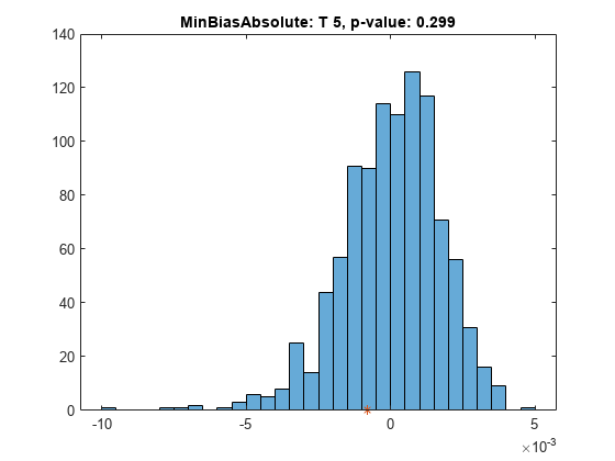
Figure contains an axes object. The axes object with title MinBiasAbsolute: T 5, p-value: 0.299 contains 2 objects of type histogram, line. One or more of the lines displays its values using only markers

The unconditional test statistic reported by esbacktestbysim is exactly the same as the unconditional test statistic reported by esbacktest. However the critical values reported by esbacktestbysim are based on a simulation using a t distribution with 5 degrees of freedom and the given location and scale parameters. The esbacktest object gives approximate test results for the "T 5" model, whereas the results here are specific for the distribution information provided. Also, for the conditional test, this is a visualization of the standalone conditional test (ConditionalOnly result in the table above). The final conditional test result (Conditional column) depends also on a preliminary VaR backtest (VaRTestResult column).

The "T 5" model is accepted by the five tests.

The esbacktestbysim object provides a simulate function to run a new simulation. For example, if there is a borderline test result where the test statistic is near the critical value, you might use the simulate function to simulate new scenarios. In cases where more precision is required, a larger simulation can be run.

The esbacktestbysim tests can be run over a rolling window, following the same approach described above for esbacktest. User-defined traffic-light tests can also be defined, for example, using two different test confidence levels, similar to what was done above for esbacktest.

Large-Sample and Simulation Tests

The esbacktestbyde object supports two ES back tests with critical values determined either with a large-sample approximation or a simulation (finite sample). esbacktestbyde requires the distribution information for the portfolio outcomes, namely, the distribution name ("normal" or "t") and the distribution parameters for each day in the test window. It does not require the VaR of the ES data. esbacktestbyde uses the provided distribution information to map the portfolio outcomes into "ranks", that is, to apply the cumulative distribution function to map returns into values in the unit interval, where the test statistics are defined. esbacktestbyde can determine critical values by using a large-sample approximation or a finite-sample simulation.

The tests supported in esbacktestbyde are conditionalDE and unconditionalDE. These are implementations of the tests proposed by Du and Escanciano in [3]. The unconditionalDE tests and all the tests previously discussed in this example are severity tests that assess if the magnitude of the tail losses is consistent with the model predictions. The conditionalDE test, however, is a test for independence over time that assess if there is evidence of autocorrelation in the series of tail losses.

The esbacktestbyde object supports normal and t distributions. These tests can be used for any model where the underlying distribution of portfolio outcomes is normal or t, such as exponentially weighted moving average (EWMA), delta-gamma, or generalized autoregressive conditional heteroskedasticity (GARCH) models.

The "Normal", "T 10", and "T 5" models can be backtested with the tests in esbacktestbyde. For illustration purposes, only "T 5" is backtested. The distribution name ("t") and parameters (DegreesOfFreedom, Location, and Scale) are provided when the esbacktestbyde object is created.

rng('default'); % for reproducibility; the esbacktestbyde constructor runs a simulation
ebtde = esbacktestbyde(ReturnsTest,"t",'DegreesOfFreedom',5,...
   'Location',Mu,'Scale',SigmaT5,...
   'PortfolioID',"S&P",'VaRID',"T 5",'VaRLevel',VaRLevel);

The recommended workflow is the same: first, run the summary function, then run the runtests function, and then run the individual test functions. The summary function provides exactly the same information as the summary function from esbacktest.

s = summary(ebtde);
disp(s)

    PortfolioID    VaRID    VaRLevel    ObservedLevel    ExpectedSeverity    ObservedSeverity    Observations    Failures    Expected    Ratio     Missing
    ___________    _____    ________    _____________    ________________    ________________    ____________    ________    ________    ______    _______

       "S&P"       "T 5"     0.975         0.97173             1.37               1.4075             2087           59        52.175     1.1308       0

The runtests function shows the final accept or reject result.

t = runtests(ebtde);
disp(t)

    PortfolioID    VaRID    VaRLevel    ConditionalDE    UnconditionalDE
    ___________    _____    ________    _____________    _______________

       "S&P"       "T 5"     0.975         reject            accept

Additional details on the test results are obtained by calling the individual test functions.

t = conditionalDE(ebtde);
disp(t)

    PortfolioID    VaRID    VaRLevel    ConditionalDE      PValue      TestStatistic    CriticalValue    AutoCorrelation    Observations    CriticalValueMethod    NumLags    Scenarios    TestLevel
    ___________    _____    ________    _____________    __________    _____________    _____________    _______________    ____________    ___________________    _______    _________    _________

       "S&P"       "T 5"     0.975         reject        0.00034769       12.794           3.8415           0.078297            2087          "large-sample"          1          NaN         0.95

By default, the critical values are determined by a large-sample approximation. Critical values based on a finite-sample distribution estimated by using a simulation are available when using the 'CriticalValueMethod' optional name-value pair argument.

[t,s] = conditionalDE(ebtde,'CriticalValueMethod','simulation');
disp(t)

    PortfolioID    VaRID    VaRLevel    ConditionalDE    PValue    TestStatistic    CriticalValue    AutoCorrelation    Observations    CriticalValueMethod    NumLags    Scenarios    TestLevel
    ___________    _____    ________    _____________    ______    _____________    _____________    _______________    ____________    ___________________    _______    _________    _________

       "S&P"       "T 5"     0.975         reject         0.01        12.794           3.7961           0.078297            2087           "simulation"           1         1000         0.95

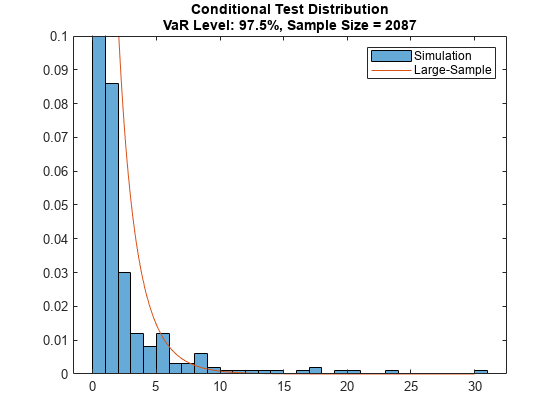
The second output, s, contains simulated test statistic values. The following visualization is useful for comparing how well the simulated finite-sample distribution matches the large-sample approximation. The plot shows that the tail of the distribution of test statistics is slightly heavier for the simulation-based (finite-sample) distribution. This means the simulation-based version of the tests are more tolerant and would not reject in some cases where the large-sample approximation results reject. How closely the large-sample and simulation distributions match depends not only on the number of observations in the test window, but also on the VaR confidence level (higher VaR levels lead to heavier tails in the finite-sample distribution).

xLS = 0:0.05:30;
pdfLS = chi2pdf(xLS,t.NumLags);
histogram(s,'Normalization',"pdf")
hold on
plot(xLS,pdfLS)
hold off
ylim([0 0.1])
legend({'Simulation','Large-Sample'})
Title = sprintf('Conditional Test Distribution\nVaR Level: %g%%, Sample Size = %d',VaRLevel*100,t.Observations);
title(Title)

Figure contains an axes object. The axes object with title Conditional Test Distribution VaR Level: 97.5%, Sample Size = 2087 contains 2 objects of type histogram, line. These objects represent Simulation, Large-Sample.

Similar steps can be used to see details on the unconditionalDE test, and to compare the large-sample and simulation based results.

The esbacktestbyde object provides a simulate function to run a new simulation. For example, if there is a borderline test result where the test statistic is near the critical value, you can use the simulate function to simulate new scenarios. Also, by default, the simulation stores results for up to 5 lags for the conditional test, so if simulation-based results for a larger number of lags is needed, you must use the simulate function.

If the large-sample approximation tests are the only tests that you need because they are reliable for a particular sample size and VaR level, you can turn off simulation when creating an esbacktestbyde object by using the 'Simulate' optional input.

The esbacktestbyde tests can be run over a rolling window, following the same approach described above for esbacktest. You can also define traffic-light tests, for example, you could use two different test confidence levels, similar to what was done above for esbacktest.

Conclusions

To contrast the three ES backtesting objects:

The esbacktest object is used for a wide range of distributional assumptions: historical VaR, parametric VaR, Monte-Carlo VaR, or extreme-value models. However, esbacktest offers approximate test results based on two variations of the same test: the unconditional test statistic with two different sets of precomputed critical values (unconditionalNormal and unconditionalT).
The esbacktestbysim object is used for parametric methods with normal and t distributions (which includes EWMA, GARCH, and delta-gamma) and requires distribution parameters as inputs. esbacktestbysim offers five different tests (conditional, unconditional, quantile, minBiasAbsolute, and minBiasRelative and the critical values for these tests are simulated using the distribution information that you provide, and therefore, are more accurate. Although all ES backtests are sensitive to VaR estimation errors, the minimally biased test has only a small sensitivity and is recommended (see Acerbi-Szekely 2017 and 2019 for details [2], [3]).
The esbacktestbyde object is also used for parametric methods with normal and t distributions (which includes EWMA, GARCH, and delta-gamma) and requires distribution parameters as inputs. esbacktestbyde contains a severity (unconditionalDE) and a time-independence (conditionalDE) tests and it has the convenience of a large-sample, fast version of the tests. The conditionalDE test is the only test for independence over time for ES models among all the tests supported in these three classes.

As shown in this example, all three ES backtesting objects provide functionality to generate reports on severities, VaR failures, and test results information. The three ES backtest objects provide the flexibility to build on them. For example, you can create user-defined traffic-light tests and run the ES backtesting analysis over rolling windows.

References

[1] Acerbi, C., and B. Szekely. "Backtesting Expected Shortfall." MSCI Inc., December 2014.

[2] Acerbi, C., and B. Szekely. "General Properties of Backtestable Statistics. SSRN Electronic Journal. January, 2017.

[3] Acerbi, C., and B. Szekely. "The Minimally Biased Backtest for ES." Risk. September, 2019.

[4] Basel Committee on Banking Supervision. "Minimum Capital Requirements for Market Risk." January 2016, https://www.bis.org/bcbs/publ/d352.htm

[5] Du, Z., and J. C. Escanciano. "Backtesting Expected Shortfall: Accounting for Tail Risk." Management Science. Vol 63, Issue 4, April 2017.

[6] McNeil, A., R. Frey, and P. Embrechts. Quantitative Risk Management: Concepts, Techniques and Tools. Princeton University Press. 2005.

[7] Rockafellar, R. T. and S. Uryasev. "Conditional Value-at-Risk for General Loss Distributions." Journal of Banking and Finance. Vol. 26, 2002, pp. 1443-1471.

Local Functions

function [VaR,ES] = hHistoricalVaRES(Sample,VaRLevel)
    % Compute historical VaR and ES
    % See [7] for technical details

    % Convert to losses
    Sample = -Sample;
    
    N = length(Sample);
    k = ceil(N*VaRLevel);
    
    z = sort(Sample);
    
    VaR = z(k);
    
    if k < N
       ES = ((k - N*VaRLevel)*z(k) + sum(z(k+1:N)))/(N*(1 - VaRLevel));
    else
       ES = z(k);
    end
end

function [VaR,ES] = hNormalVaRES(Mu,Sigma,VaRLevel)
    % Compute VaR and ES for normal distribution
    % See [6] for technical details
    
    VaR = -1*(Mu-Sigma*norminv(VaRLevel));
    ES = -1*(Mu-Sigma*normpdf(norminv(VaRLevel))./(1-VaRLevel));

end

function [VaR,ES] = hTVaRES(DoF,Mu,Sigma,VaRLevel)
    % Compute VaR and ES for t location-scale distribution
    % See [6] for technical details

    VaR = -1*(Mu-Sigma*tinv(VaRLevel,DoF));
    ES_StandardT = (tpdf(tinv(VaRLevel,DoF),DoF).*(DoF+tinv(VaRLevel,DoF).^2)./((1-VaRLevel).*(DoF-1)));
    ES = -1*(Mu-Sigma*ES_StandardT);

end

Related Examples

More About

Overview of Expected Shortfall Backtesting