Working with Big Data

Financial markets, with electronic exchanges such as NASDAQ executing orders on a timescale of milliseconds, generate vast amounts of data. Data streams can be mined for statistical arbitrage opportunities, but traditional methods for processing and storing dynamic analytic information can be overwhelmed by big data. Fortunately, new computational approaches have emerged, and MATLAB has an array of tools for implementing them.

Main computer memory provides high-speed access but limited capacity, whereas external storage offers low-speed access but potentially unlimited capacity. Computation takes place in memory. The computer recalls data and results from external storage.

Data Files

This example uses one trading day of NASDAQ exchange data [2] on one security (INTC) in a sample provided by LOBSTER [1] and included with Financial Toolbox™ documentation in the zip file LOBSTER_SampleFile_INTC_2012-06-21_5.zip. Extract the contents of the zip file into your current folder. The expanded files, including two CSV files of data and the text file LOBSTER_SampleFiles_ReadMe.txt, consume 93.7 MB of memory.

unzip("LOBSTER_SampleFile_INTC_2012-06-21_5.zip");

The data describes the intraday evolution of the limit order book (LOB), which is the record of market orders (best price), limit orders (designated price), and resulting buys and sells. The data includes the precise time of these events, with orders tracked from arrival until cancellation or execution. At each moment in the trading day, orders on both the buy and sell side of the LOB exist at various levels away from the midprice between the lowest ask (order to sell) and the highest bid (order to buy).

Level 5 data (five levels away from the midprice on either side) is contained in two CSV files. Extract the trading date from the message file name.

MSGFileName = "INTC_2012-06-21_34200000_57600000_message_5.csv";   % Message file (description of data)
LOBFileName = "INTC_2012-06-21_34200000_57600000_orderbook_5.csv"; % Data file

[ticker,rem] = strtok(MSGFileName,'_');
date = strtok(rem,'_'); 

Data Storage

Daily data streams accumulate and need to be stored. A datastore is a repository for collections of data that are too big to fit in memory.

Use tabularTextDatastore to create datastores for the message and data files. Because the files contain data with different formats, create the datastores separately. Ignore generic column headers (for example, VarName1) by setting the 'ReadVariableNames' name-value argument to false. Replace the headers with descriptive variable names obtained from LOBSTER_SampleFiles_ReadMe.txt. Set the 'ReadSize' name-value argument to 'file' to allow similarly formatted files to be appended to existing datastores at the end of each trading day.

DSMSG = tabularTextDatastore(MSGFileName,'ReadVariableNames',false,'ReadSize','file');
DSMSG.VariableNames = ["Time","Type","OrderID","Size","Price","Direction"];

DSLOB = tabularTextDatastore(LOBFileName,'ReadVariableNames',false,'ReadSize','file');
DSLOB.VariableNames = ["AskPrice1","AskSize1","BidPrice1","BidSize1",...
                       "AskPrice2","AskSize2","BidPrice2","BidSize2",...
                       "AskPrice3","AskSize3","BidPrice3","BidSize3",...
                       "AskPrice4","AskSize4","BidPrice4","BidSize4",...
                       "AskPrice5","AskSize5","BidPrice5","BidSize5"];

Create a combined datastore by selecting Time and the level 3 data.

TimeVariable = "Time";
DSMSG.SelectedVariableNames = TimeVariable;

LOB3Variables = ["AskPrice1","AskSize1","BidPrice1","BidSize1",...
                 "AskPrice2","AskSize2","BidPrice2","BidSize2",...
                 "AskPrice3","AskSize3","BidPrice3","BidSize3"];
DSLOB.SelectedVariableNames = LOB3Variables;
                               
DS = combine(DSMSG,DSLOB);         

You can preview the first few rows in the combined datastore without loading data into memory.

DSPreview = preview(DS);
LOBPreview = DSPreview(:,1:5)

LOBPreview=8×5 table
    Time     AskPrice1    AskSize1    BidPrice1    BidSize1
    _____    _________    ________    _________    ________

    34200    2.752e+05       66       2.751e+05      400   
    34200    2.752e+05      166       2.751e+05      400   
    34200    2.752e+05      166       2.751e+05      400   
    34200    2.752e+05      166       2.751e+05      400   
    34200    2.752e+05      166       2.751e+05      300   
    34200    2.752e+05      166       2.751e+05      300   
    34200    2.752e+05      166       2.751e+05      300   
    34200    2.752e+05      166       2.751e+05      300   

The preview shows asks and bids at the touch, meaning the level 1 data, which is closest to the midprice. Time units are seconds after midnight, price units are dollar amounts times 10,000, and size units are the number of shares (see LOBSTER_SampleFiles_ReadMe.txt).

Tall Arrays and Timetables

Tall arrays work with out-of-memory data backed by a datastore using the MapReduce technique (see Tall Arrays for Out-of-Memory Data). When you use MapReduce, tall arrays remain unevaluated until you execute specific computations that use the data.

Set the execution environment for MapReduce to the local MATLAB session, instead of using Parallel Computing Toolbox™, by calling mapreducer(0). Then, create a tall array from the datastore DS by using tall. Preview the data in the tall array.

mapreducer(0)
DT = tall(DS);

DTPreview = DT(:,1:5)

DTPreview =

  Mx5 tall table

    Time     AskPrice1    AskSize1    BidPrice1    BidSize1
    _____    _________    ________    _________    ________

    34200    2.752e+05       66       2.751e+05      400   
    34200    2.752e+05      166       2.751e+05      400   
    34200    2.752e+05      166       2.751e+05      400   
    34200    2.752e+05      166       2.751e+05      400   
    34200    2.752e+05      166       2.751e+05      300   
    34200    2.752e+05      166       2.751e+05      300   
    34200    2.752e+05      166       2.751e+05      300   
    34200    2.752e+05      166       2.751e+05      300   
      :          :           :            :           :
      :          :           :            :           :

Timetables allow you to perform operations specific to time series (see Create Timetables). Because the LOB data consists of concurrent time series, convert DT to a tall timetable.

DT.Time = seconds(DT.Time); % Cast time as a duration from midnight.
DTT = table2timetable(DT);

DTTPreview = DTT(:,1:4)

DTTPreview =

  Mx4 tall timetable

      Time       AskPrice1    AskSize1    BidPrice1    BidSize1
    _________    _________    ________    _________    ________

    34200 sec    2.752e+05       66       2.751e+05      400   
    34200 sec    2.752e+05      166       2.751e+05      400   
    34200 sec    2.752e+05      166       2.751e+05      400   
    34200 sec    2.752e+05      166       2.751e+05      400   
    34200 sec    2.752e+05      166       2.751e+05      300   
    34200 sec    2.752e+05      166       2.751e+05      300   
    34200 sec    2.752e+05      166       2.751e+05      300   
    34200 sec    2.752e+05      166       2.751e+05      300   
        :            :           :            :           :
        :            :           :            :           :

Display all variables in the MATLAB workspace.

whos

  Name               Size            Bytes  Class                                       Attributes

  DS                 1x1                 8  matlab.io.datastore.CombinedDatastore                 
  DSLOB              1x1                 8  matlab.io.datastore.TabularTextDatastore              
  DSMSG              1x1                 8  matlab.io.datastore.TabularTextDatastore              
  DSPreview          8x13             4515  table                                                 
  DT                 Mx13             4950  tall                                                  
  DTPreview          Mx5              2840  tall                                                  
  DTT                Mx12             4746  tall                                                  
  DTTPreview         Mx4              2650  tall                                                  
  LOB3Variables      1x12              780  string                                                
  LOBFileName        1x1               234  string                                                
  LOBPreview         8x5              2203  table                                                 
  MSGFileName        1x1               230  string                                                
  TimeVariable       1x1               150  string                                                
  date               1x1               156  string                                                
  rem                1x1               222  string                                                
  ticker             1x1               150  string                                                

Because all the data is in the datastore, the workspace uses little memory.

Preprocess and Evaluate Data

Tall arrays allow preprocessing, or queuing, of computations before they are evaluated, which improves memory management in the workspace.

Midprice S and imbalance index I are used to model LOB dynamics. To queue their computations, define them, and the time base, in terms of DTT.

timeBase = DTT.Time;
MidPrice = (DTT.BidPrice1 + DTT.AskPrice1)/2;

% LOB level 3 imbalance index:

lambda  = 0.5; % Hyperparameter
weights = exp(-(lambda)*[0 1 2]);
VAsk = weights(1)*DTT.AskSize1 + weights(2)*DTT.AskSize2 + weights(3)*DTT.AskSize3;
VBid = weights(1)*DTT.BidSize1 + weights(2)*DTT.BidSize2 + weights(3)*DTT.BidSize3;
ImbalanceIndex = (VBid-VAsk)./(VBid+VAsk);

The imbalance index is a weighted average of ask and bid volumes on either side of the midprice [3]. The imbalance index is a potential indicator of future price movements. The variable lambda is a hyperparameter, which is a parameter specified before training rather than estimated by the machine learning algorithm. A hyperparameter can influence the performance of the model. Feature engineering is the process of choosing domain-specific hyperparameters to use in machine learning algorithms. You can tune hyperparameters to optimize a trading strategy.

To bring preprocessed expressions into memory and evaluate them, use the gather function. This process is called deferred evaluation.

[t,S,I] = gather(timeBase,MidPrice,ImbalanceIndex);

Evaluating tall expression using the Local MATLAB Session:
- Pass 1 of 1: Completed in 1.2 sec
Evaluation completed in 1.3 sec

A single call to gather evaluates multiple preprocessed expressions with a single pass through the datastore.

Determine the sample size, which is the number of ticks, or updates, in the data.

numTicks = length(t)

numTicks = 581030

The daily LOB data contains 581,030 ticks.

Checkpoint Data

You can save both unevaluated and evaluated data to external storage for later use.

Prepend the time base with the date, and cast the result as a datetime array. Save the resulting datetime array, MidPrice, and ImbalanceIndex to a MAT-file in a specified location.

dateTimeBase = datetime(date) + timeBase; 
Today = timetable(dateTimeBase,MidPrice,ImbalanceIndex)

Today =

  581,030x2 tall timetable

        dateTimeBase         MidPrice     ImbalanceIndex
    ____________________    __________    ______________

    21-Jun-2012 09:30:00    2.7515e+05         -0.205   
    21-Jun-2012 09:30:00    2.7515e+05       -0.26006   
    21-Jun-2012 09:30:00    2.7515e+05       -0.26006   
    21-Jun-2012 09:30:00    2.7515e+05      -0.086772   
    21-Jun-2012 09:30:00    2.7515e+05       -0.15581   
    21-Jun-2012 09:30:00    2.7515e+05       -0.35382   
    21-Jun-2012 09:30:00    2.7515e+05       -0.19084   
    21-Jun-2012 09:30:00    2.7515e+05       -0.19084   
             :                  :               :
             :                  :               :

location = fullfile(pwd,"ExchangeData",ticker,date);
write(location,Today,'FileType','mat')

Writing tall data to folder /tmp/Bdoc23b_2361005_2898260/tp322fef83/finance-ex97702880/ExchangeData/INTC/2012-06-21
Evaluating tall expression using the Local MATLAB Session:
- Pass 1 of 1: Completed in 1.7 sec
Evaluation completed in 1.8 sec

The file is written once, at the end of each trading day. The code saves the data to a file in a date-stamped folder. The series of ExchangeData subfolders serves as a historical data repository.

Alternatively, you can save workspace variables evaluated with gather directly to a MAT-file in the current folder.

save("LOBVars.mat","t","S","I")

In preparation for model validation later on, evaluate and add market order prices to the same file.

[MOBid,MOAsk] = gather(DTT.BidPrice1,DTT.AskPrice1);

Evaluating tall expression using the Local MATLAB Session:
- Pass 1 of 1: Completed in 1 sec
Evaluation completed in 1 sec

save("LOBVars.mat","MOBid","MOAsk","-append")

The remainder of this example uses only the unevaluated tall timetable DTT. Clear other variables from the workspace.

clearvars -except DTT 
whos

  Name            Size            Bytes  Class    Attributes

  DTT       581,030x12             4746  tall               

Data Visualization

To visualize large amounts of data, you must summarize, bin, or sample the data in some way to reduce the number of points plotted on the screen.

LOB Snapshot

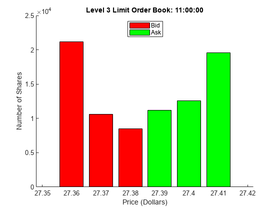
One method of visualization is to evaluate only a selected subsample of the data. Create a snapshot of the LOB at a specific time of day (11 AM).

sampleTimeTarget = seconds(11*60*60);               % Seconds after midnight
sampleTimes = withtol(sampleTimeTarget,seconds(1)); % 1 second tolerance
sampleLOB = DTT(sampleTimes,:);

numTimes = gather(size(sampleLOB,1))

Evaluating tall expression using the Local MATLAB Session:
- Pass 1 of 1: Completed in 1.1 sec
Evaluation completed in 1.2 sec

numTimes = 23

There are 23 ticks within one second of 11 AM. For the snapshot, use the tick closest to the midtime.

sampleLOB = sampleLOB(round(numTimes/2),:);
sampleTime = sampleLOB.Time;

sampleBidPrices = [sampleLOB.BidPrice1,sampleLOB.BidPrice2,sampleLOB.BidPrice3];
sampleBidSizes  = [sampleLOB.BidSize1,sampleLOB.BidSize2,sampleLOB.BidSize3];
sampleAskPrices = [sampleLOB.AskPrice1,sampleLOB.AskPrice2,sampleLOB.AskPrice3];
sampleAskSizes  = [sampleLOB.AskSize1,sampleLOB.AskSize2,sampleLOB.AskSize3];

[sampleTime,sampleBidPrices,sampleBidSizes,sampleAskPrices,sampleAskSizes] = ...
    gather(sampleTime,sampleBidPrices,sampleBidSizes,sampleAskPrices,sampleAskSizes);

Evaluating tall expression using the Local MATLAB Session:
- Pass 1 of 2: Completed in 1 sec
- Pass 2 of 2: Completed in 1.1 sec
Evaluation completed in 2.4 sec

Visualize the limited data sample returned by gather by using bar.

figure
hold on

bar((sampleBidPrices/10000),sampleBidSizes,'r')
bar((sampleAskPrices/10000),sampleAskSizes,'g')
hold off

xlabel("Price (Dollars)")
ylabel("Number of Shares")
legend(["Bid","Ask"],'Location','North')
title(strcat("Level 3 Limit Order Book: ",datestr(sampleTime,"HH:MM:SS")))

Depth of Market

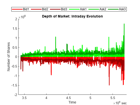
Some visualization functions work directly with tall arrays and do not require the use of gather (see Visualization of Tall Arrays). The functions automatically sample data to decrease pixel density. Visualize the level 3 intraday depth of market, which shows the time evolution of liquidity, by using plot with the tall timetable DTT.

figure
hold on

plot(DTT.Time,-DTT.BidSize1,'Color',[1.0 0 0],'LineWidth',2)
plot(DTT.Time,-DTT.BidSize2,'Color',[0.8 0 0],'LineWidth',2)
plot(DTT.Time,-DTT.BidSize3,'Color',[0.6 0 0],'LineWidth',2)

plot(DTT.Time,DTT.AskSize1,'Color',[0 1.0 0],'LineWidth',2)
plot(DTT.Time,DTT.AskSize2,'Color',[0 0.8 0],'LineWidth',2)
plot(DTT.Time,DTT.AskSize3,'Color',[0 0.6 0],'LineWidth',2)

hold off

xlabel("Time")
ylabel("Number of Shares")
title("Depth of Market: Intraday Evolution")
legend(["Bid1","Bid2","Bid3","Ask1","Ask2","Ask3"],'Location','NorthOutside','Orientation','Horizontal');

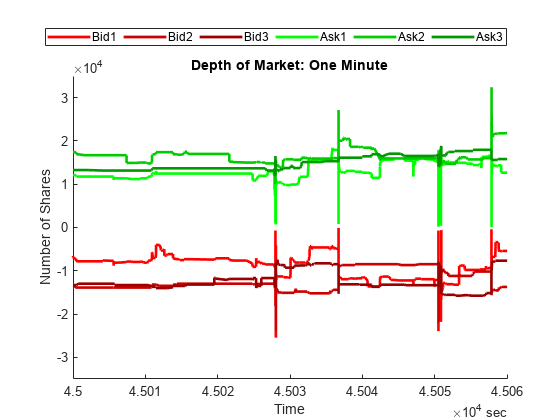
To display details, limit the time interval.

xlim(seconds([45000 45060]))
ylim([-35000 35000])
title("Depth of Market: One Minute")

Summary

This example introduces the basics of working with big data, both in and out of memory. It shows how to set up, combine, and update external datastores, then create tall arrays for preprocessing data without allocating variables in the MATLAB workspace. The gather function transfers data into the workspace for computation and further analysis. The example shows how to visualize the data through data sampling or by MATLAB plotting functions that work directly with out-of-memory data.