littlewoodPaleySum
Syntax
Description
[
returns the Littlewood-Paley sums for the first- and second-order wavelet time filter banks,
lpsum1,lpsum2] = littlewoodPaleySum(jtfn)lpsum1 and lpsum2 respectively, in the joint
time-frequency scattering (JTFS) network, jtfn.
For more information about the Littlewood-Paley sums, see Proposition 2.1 in [1].
[
returns the Littlewood-Paley sums for the lpsum1,lpsum2] = littlewoodPaleySum(jtfn,FilterBank=filterbanktype)filterbanktype filter
banks.
Examples
Littlewood-Paley Sums of JTFS Network
Use timeFrequencyScattering with default settings to create a joint time-frequency scattering (JTFS) network.
jtfn = timeFrequencyScattering;
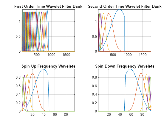
Plot the wavelet filters in the first- and second-order time filter banks, and the spin-up and spin-down wavelet filters. The filter magnitudes are not equal because, by default, the network attempts to approximate the Littlewood-Paley condition for the filters. You can change this default behavior through the EnergyCorrectFilters network property.
[psi1f,psi2f,~] = filterbank(jtfn);
[psiffrup,psiffrdn,~] = filterbank(jtfn,FilterBank="frequency");
tiledlayout(2,2)
nexttile
plot(psi1f)
grid on
axis tight
title("First-Order Time Wavelet Filter Bank")
nexttile
plot(psi2f)
grid on
axis tight
title("Second-Order Time Wavelet Filter Bank")
nexttile
plot(psiffrup)
grid on
title("Spin-Up Frequency Wavelets")
axis tight
nexttile
plot(psiffrdn)
title("Spin-Down Frequency Wavelets")
grid on
axis tight
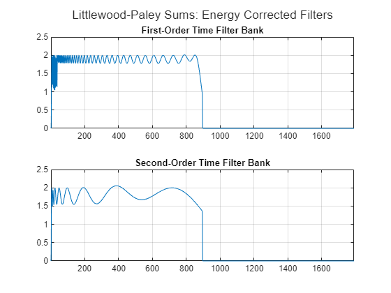
To see the effect of the approximation, use littlewoodPaleySum to plot the Littlewood-Paley sums of the first- and second-order time filter banks. In the theoretical best-case scenario, the Littlewood-Paley sum for these filters is a straight line equal to 2 from 0 to the Nyquist, and zero after that. Given the freedom you have in constructing the network, the best-case scenario is not possible. Therefore, the network approximates the filters so that the Littlewood-Paley sums are as close to 2 as possible.
[lpsum1,lpsum2] = littlewoodPaleySum(jtfn,FilterBank="time");
figure
t = tiledlayout(2,1);
nexttile
plot(lpsum1)
title("First-Order Time Filter Bank")
grid on
xlim([1 numel(lpsum1)])
nexttile
plot(lpsum2)
title("Second-Order Time Filter Bank")
xlim([1 numel(lpsum2)])
grid on
title(t,"Littlewood-Paley Sums: Energy Corrected Filters")
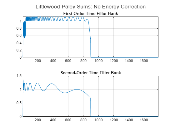
To see the impact of the energy correction, create a JTFS network with EnergyCorrectFilters set to false. Plot the Littlewood-Paley sums of the wavelet time filter banks. These sums are very different from the sums of the energy-corrected filters and far below the expected theoretical value of 2.
jtfn = timeFrequencyScattering(EnergyCorrectFilters=false);
[lpsum1,lpsum2] = littlewoodPaleySum(jtfn,FilterBank="time");
figure
t = tiledlayout(2,1);
nexttile
plot(lpsum1)
title("First-Order Time Filter Bank")
grid on
xlim([1 numel(lpsum1)])
nexttile
plot(lpsum2)
title("Second-Order Time Filter Bank")
xlim([1 numel(lpsum2)])
grid on
title(t,"Littlewood-Paley Sums: No Energy Correction")
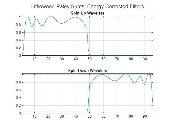
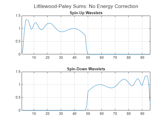
Repeat the same steps for the spin-up and spin-down wavelet filters. In the theoretical best-case scenario, the Littlewood-Paley sum for these filters would be a straight line equal to 1 across the entire range. As is the case for the time wavelet filters, it is not possible to achieve this theoretical value exactly.
Plot the Littlewood-Paley sums of the spin-up and spin-down wavelets in the default JTFS network.
jtfn = timeFrequencyScattering;
[lpsum1,lpsum2] = littlewoodPaleySum(jtfn,FilterBank="frequency");
figure
t = tiledlayout(2,1);
nexttile
plot(lpsum1)
title("Spin-Up Wavelets")
grid on
xlim([1 numel(lpsum1)])
nexttile
plot(lpsum2)
title("Spin-Down Wavelets")
xlim([1 numel(lpsum2)])
grid on
title(t,"Littlewood-Paley Sums: Energy Corrected Filters")
Compare with a plot of the Littlewood-Paley sums using a JTFS network with EnergyCorrectFilters set to false. Without energy correction, the sums oscillate significantly above and below the expected theoretical value of 1. The sums of the spin-up and spin-down wavelets also exhibit downward and upward trends, respectively. This behavior does not occur for the energy-corrected filters.
jtfn = timeFrequencyScattering(EnergyCorrectFilters=false);
[lpsum1,lpsum2] = littlewoodPaleySum(jtfn,FilterBank="frequency");
figure
t = tiledlayout(2,1);
nexttile
plot(lpsum1)
title("Spin-Up Wavelets")
grid on
xlim([1 numel(lpsum1)])
nexttile
plot(lpsum2)
title("Spin-Down Wavelets")
xlim([1 numel(lpsum2)])
grid on
title(t,"Littlewood-Paley Sums: No Energy Correction")
Input Arguments
jtfn — Joint time-frequency scattering network
timeFrequencyScattering object
Joint time-frequency scattering network, specified as a timeFrequencyScattering object.
filterbanktype — Filter banks type
"time" (default) | "frequency"
Filter banks type, specified as one of the following:
"time"— First- and second-order wavelet time filter banks"frequency"— Spin-up and spin-down wavelet filters
Output Arguments
lpsum1 — Littlewood-Paley sum
vector
Littlewood-Paley sum of the first filterbanktype filter bank.
If filterbanktype is "time", the sum is of the
first-order wavelet time filter bank. If filterbanktype is
"frequency", the sum is of the spin-up wavelet filters.
lpsum2 — Littlewood-Paley sum
vector
Littlewood-Paley sum of the second filterbanktype filter bank.
If filterbanktype is "time", the sum is of the
second-order wavelet time filter bank. If filterbanktype is
"frequency", the sum is of the spin-down wavelet filters.
References
[1] Mallat, Stéphane. “Group Invariant Scattering.” Communications on Pure and Applied Mathematics 65, no. 10 (October 2012): 1331–98. https://doi.org/10.1002/cpa.21413
Version History
Introduced in R2024b
MATLAB Command
You clicked a link that corresponds to this MATLAB command:
Run the command by entering it in the MATLAB Command Window. Web browsers do not support MATLAB commands.

Select a Web Site
Choose a web site to get translated content where available and see local events and offers. Based on your location, we recommend that you select: .
You can also select a web site from the following list
How to Get Best Site Performance
Select the China site (in Chinese or English) for best site performance. Other bat365 country sites are not optimized for visits from your location.
Americas
- América Latina (Español)
- Canada (English)
- United States (English)
Europe
- Belgium (English)
- Denmark (English)
- Deutschland (Deutsch)
- España (Español)
- Finland (English)
- France (Français)
- Ireland (English)
- Italia (Italiano)
- Luxembourg (English)
- Netherlands (English)
- Norway (English)
- Österreich (Deutsch)
- Portugal (English)
- Sweden (English)
- Switzerland
- United Kingdom (English)
Asia Pacific
- Australia (English)
- India (English)
- New Zealand (English)
- 中国
- 日本Japanese (日本語)
- 한국Korean (한국어)