filterbank
Syntax
Description
[
returns the spin-up and spin-down frequency wavelets, psifup,psifdown,phiffr,frequencymeta] = filterbank(jtfn,FilterBank="frequency")psifup and
psifdown respectively, the frequency lowpass filter
phiffr, and the metadata frequencymeta for the
frequency filters in the JTFS network.
The syntax filterbank(jtfn,FilterBank="time") is equivalent to
filterbank(jtfn).
Examples
Obtain JTFS Time Wavelet Filter Banks
Create a JTFS network with the energy correct filters option set to false. Specify quality factors of 9 and 2 for the first-order and second-order time wavelet filter banks, respectively.
jtfn = timeFrequencyScattering(EnergyCorrectFilters=false, ...
    TimeQualityFactors=[9 2]);
Obtain the filters in the first- and second-order time wavelet filter banks and their metadata. Plot the filters. Because the wavelets are analytic, their Fourier transforms are supported only on the positive real axis.
[psi1f,psi2f,phift,timemeta] = filterbank(jtfn);
tiledlayout(2,1)
nexttile
plot(psi1f)
grid on
axis tight
title("First-Order Time Wavelet Filter Bank")
nexttile
plot(psi2f)
grid on
axis tight
title("Second-Order Time Wavelet Filter Bank")
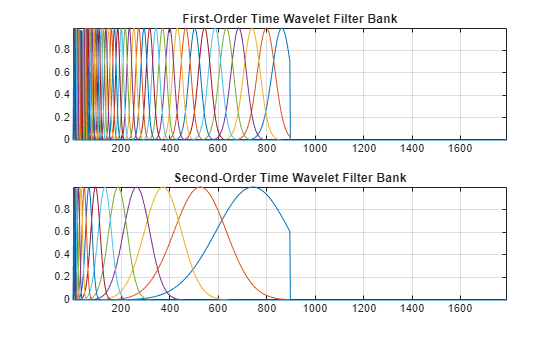
Inspect the size and metadata for the first-order time wavelet filter bank. The wavelet filters are arranged columnwise and in order of decreasing center frequency. The th table row describes the th filter.
size(psi1f)
ans = 1×2

        1792          50
timemeta{1}ans=50×6 table
xi sigma isCQT log2dsfactor peakidx bwidx
_______ _________ _____ ____________ _______ __________
0.48076 0.022225 1 0 863 757 897
0.44512 0.020578 1 0 799 701 896
0.41212 0.019053 1 0 740 646 833
0.38158 0.01764 1 0 685 598 771
0.35329 0.016333 1 0 634 553 714
0.3271 0.015122 1 0 587 512 661
0.30286 0.014001 1 0 544 475 613
0.28041 0.012963 1 0 503 440 567
0.25962 0.012002 1 0 466 407 525
0.24038 0.011113 1 0 432 377 486
0.22256 0.010289 1 0 400 349 450
0.20606 0.0095263 1 1 370 324 417
0.19079 0.0088202 1 1 343 300 386
0.17665 0.0081664 1 1 318 278 358
0.16355 0.007561 1 1 294 257 331
0.15143 0.0070006 1 1 272 237 306
⋮
Choose a time filter bank. From its metadata, obtain the filter center frequencies and the logical values indicating if a center frequency is logarithmically spaced.
whichFB = 1;
centerFrq = timemeta{whichFB}.xi;
isCQT = timemeta{whichFB}.isCQT;
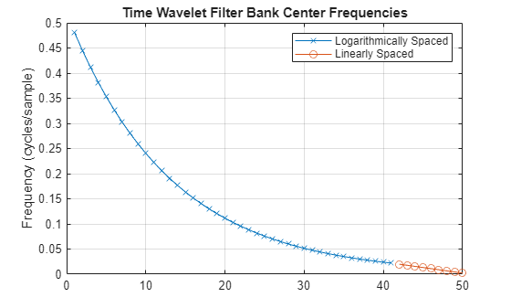
Compute the ratios of consecutive center frequencies that are logarithmically spaced. Confirm the ratios are equal to , where is the quality factor of the filter bank.
qualityFactor = jtfn.TimeQualityFactors(whichFB);
isLogSpaced = find(isCQT);
cf = centerFrq(isLogSpaced);
cfRatio = cf(2:end)./cf(1:end-1);
[min(cfRatio) max(cfRatio) 2^(-1/qualityFactor)]
ans = 1×3

    0.9259    0.9259    0.9259
Plot on a linear scale with a cross marker the center frequencies that are logarithmically spaced. Then plot with a circle marker the center frequencies that are linearly spaced.
figure
plot(isLogSpaced,cf,'x-')
hold on
isNotLogSpaced = find(~isCQT);
plot(isNotLogSpaced,centerFrq(isNotLogSpaced),'o-')
hold off
grid on
legend("Logarithmically Spaced","Linearly Spaced")
title("Time Wavelet Filter Bank Center Frequencies")
ylabel("Frequency (cycles/sample)")
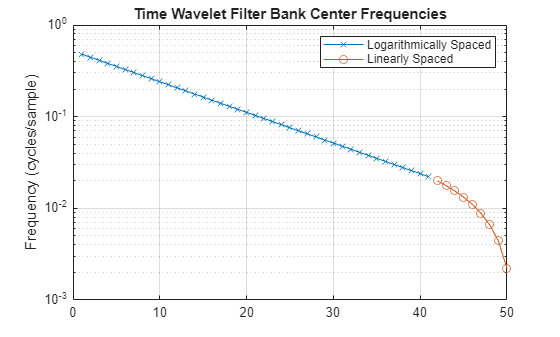
Make the same plot, but this time on a logarithmic scale.
figure
semilogy(isLogSpaced,centerFrq(isLogSpaced),'x-')
hold on
semilogy(isNotLogSpaced,centerFrq(isNotLogSpaced),'o-')
hold off
grid on
legend("Logarithmically Spaced","Linearly Spaced")
title("Time Wavelet Filter Bank Center Frequencies")
ylabel("Frequency (cycles/sample)")
Obtain JTFS Frequency Wavelet Filters
Create a JTFS network with the energy correct filters option set to false. Specify a frequency quality factor of 3.
jtfn = timeFrequencyScattering(EnergyCorrectFilters=false, ...
    FrequencyQualityFactor=3)
jtfn =
timeFrequencyScattering with properties:
SignalLength: 1024
NumFrequencyOctaves: 3
FrequencyInvarianceScale: 8
FrequencyQualityFactor: 3
TimeInvarianceScale: 128
TimeQualityFactors: [8 1]
TimeMaxPaddingFactor: 2
NumTimeOctaves: [7 7]
FilterDataType: 'double'
FrequencyMaxPaddingFactor: 2
EnergyCorrectFilters: 0
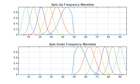
Obtain the spin-up and spin-down frequency wavelets and their metadata. Plot the wavelets.
[psifup,psifdown,phiffr,frequencymeta] = filterbank(jtfn, ...
    FilterBank="frequency");
tiledlayout(2,1)
nexttile
plot(psifup)
grid on
title("Spin-Up Frequency Wavelets")
axis tight
nexttile
plot(psifdown)
title("Spin-Down Frequency Wavelets")
grid on
axis tight
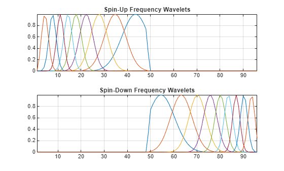
Inspect the metadata. The metadata is listed in order of decreasing center frequency, first for the spin-up wavelets, and then the spin-down wavelets.
frequencymeta
frequencymeta=18×7 table
       xi        sigma      isCQT    log2dsfactor    spin    peakidx     bwidx
    ________    ________    _____    ____________    ____    _______    ________

     0.44249    0.061128      1           0            1       43       28    49
     0.35121    0.048518      1           0            1       35       22    47
     0.27875    0.038508      1           0            1       28       18    38
     0.22125    0.030564      1           0            1       22       14    30
      0.1756    0.024259      1           1            1       18       12    24
     0.13938    0.019254      1           1            1       14       10    19
     0.10453     0.01625      0           1            1       11        7    15
    0.069688     0.01625      0           2            1        8        4    12
    0.034844     0.01625      0           2            1        4        2     8
    -0.44249    0.061128      1           0           -1       55       49    70
    -0.35121    0.048518      1           0           -1       63       51    76
    -0.27875    0.038508      1           0           -1       70       60    80
    -0.22125    0.030564      1           0           -1       76       68    84
     -0.1756    0.024259      1           1           -1       80       74    86
    -0.13938    0.019254      1           1           -1       84       79    88
    -0.10453     0.01625      0           1           -1       87       83    91
      ⋮
Obtain the center quefrencies of the spin-up wavelets and the logical value indicating if a center quefrency is logarithmically spaced.
numRows = size(frequencymeta,1);
centerQf = frequencymeta.xi(1:numRows/2);
isCQT = frequencymeta.isCQT(1:numRows/2);
Compute the ratios of consecutive center quefrencies that are logarithmically spaced. Confirm the ratios are equal to , where is the quality factor of the filter bank.
qualityFactor = jtfn.FrequencyQualityFactor;
isLogSpaced = find(isCQT);
cf = centerQf(isLogSpaced);
cfRatio = cf(2:end)./cf(1:end-1);
[min(cfRatio) max(cfRatio) 2^(-1/qualityFactor)]
ans = 1×3

    0.7937    0.7937    0.7937
By default, the number of frequency octaves is 3. Create a second network identical to the first, but instead set the number of frequency octaves to 2. Obtain the frequency wavelets and their metadata. Plot the spin-up and spin-down wavelets. The length and number of frequency wavelets is less than those in the original JTFS network.
jtfn2 = timeFrequencyScattering(EnergyCorrectFilters=false, ...
    FrequencyQualityFactor=3, ...
    NumFrequencyOctaves=2);
[psifup2,psifdown2,~,frequencymeta2] = filterbank(jtfn2, ...
    FilterBank="frequency");
tiledlayout(2,1)
nexttile
plot(psifup2)
grid on
title("Spin-Up Frequency Wavelets")
axis tight
nexttile
plot(psifdown2)
title("Spin-Down Frequency Wavelets")
grid on
axis tight
Input Arguments
jtfn — Joint time-frequency scattering network
timeFrequencyScattering object
Joint time-frequency scattering network, specified as a timeFrequencyScattering object.
Output Arguments
psi1f — First-order time wavelet filter bank
matrix
First-order time wavelet filter bank in the JTFS network, returned as a matrix. The wavelet filters are arranged columnwise and in order of decreasing center frequency.
psi2f — Second-order time wavelet filter bank
matrix
Second-order time wavelet filter bank in the JTFS network, returned as a matrix. The wavelet filters are arranged columnwise and in order of decreasing center frequency.
phift — Time lowpass filter
vector
Time lowpass filter in the JTFS network, returned as a vector.
timemeta — Time filter bank metadata
cell array
Time filter bank metadata, returned as a two-element cell array. The ith element is a MATLAB® table that describes the ith-order time filter bank. Both tables have these variables:
xi— Wavelet center frequency (cycles/sample)sigma— Frequency standard deviationisCQT— Logical value indicating if center frequency is logarithmically spacedlog2dsfactor— Maximum downsampling factor on a base-2 logarithmic scalepeakidx— Center frequency location (one-based index)bwidx— Total bandwidth used to determine maximum downsampling factor
psifup — Spin-up frequency wavelets
matrix
Spin-up frequency wavelets in the JTFS network, returned as a matrix. The wavelet filters are arranged columnwise and in order of decreasing center quefrency.
psifdown — Spin-down frequency wavelets
matrix
Spin-down frequency wavelets in the JTFS network, returned as a matrix. The wavelet filters are arranged columnwise and in order of decreasing center quefrency.
phiffr — Frequency lowpass filter
vector
Frequency lowpass filter in the JTFS network, returned as a vector.
frequencymeta — Frequency wavelet metadata
table
Frequency wavelet metadata, returned as a MATLAB table with these variables:
xi— Wavelet center quefrency (cycles/octave)sigma— Quefrency standard deviationisCQT— Logical value indicating if center quefrency is logarithmically spacedlog2dsfactor— Maximum downsampling factor on a base-2 logarithmic scalespin— Spin-up (1) or spin-down (-1) waveletpeakidx— Center quefrency location (one-based index)bwidx— Total bandwidth used to determine maximum downsampling factor
Version History
Introduced in R2024b
See Also
Objects
Functions
MATLAB Command
You clicked a link that corresponds to this MATLAB command:
Run the command by entering it in the MATLAB Command Window. Web browsers do not support MATLAB commands.

Select a Web Site
Choose a web site to get translated content where available and see local events and offers. Based on your location, we recommend that you select: .
You can also select a web site from the following list
How to Get Best Site Performance
Select the China site (in Chinese or English) for best site performance. Other bat365 country sites are not optimized for visits from your location.
Americas
- América Latina (Español)
- Canada (English)
- United States (English)
Europe
- Belgium (English)
- Denmark (English)
- Deutschland (Deutsch)
- España (Español)
- Finland (English)
- France (Français)
- Ireland (English)
- Italia (Italiano)
- Luxembourg (English)
- Netherlands (English)
- Norway (English)
- Österreich (Deutsch)
- Portugal (English)
- Sweden (English)
- Switzerland
- United Kingdom (English)
Asia Pacific
- Australia (English)
- India (English)
- New Zealand (English)
- 中国
- 日本Japanese (日本語)
- 한국Korean (한국어)