lambertw
Lambert W function
Syntax
Description
Examples
Return Equation with Lambert W Function as Its Solution
The Lambert W function W(x) is a set of
solutions of the equation x =
W(x)eW(x).
Solve this equation. The solution is the Lambert W function.
syms x W
eqn = x == W*exp(W);
solve(eqn,W)
ans =
lambertw(0, x)
Verify that branches of the Lambert W function are valid solutions of the
equation x = W*eW:
k = -2:2;
eqn = subs(eqn,W,lambertw(k,x));
isAlways(eqn)
ans =
  1×5 logical array
     1     1     1     1     1
Lambert W Function for Numeric and Symbolic Arguments
Depending on its arguments, lambertw can
return floating-point or exact symbolic results.
Compute the Lambert W functions for these numbers. Because the numbers are not symbolic objects, you get floating-point results.
A = [0 -1/exp(1); pi i];
lambertw(A)
ans =
   0.0000 + 0.0000i  -1.0000 + 0.0000i
   1.0737 + 0.0000i   0.3747 + 0.5764i
lambertw(-1,A)
ans =
     -Inf + 0.0000i  -1.0000 + 0.0000i
  -0.3910 - 4.6281i  -1.0896 - 2.7664i
Compute the Lambert W functions for the numbers converted to symbolic objects.
For most symbolic (exact) numbers, lambertw returns unresolved
symbolic calls.
A = [0 -1/exp(sym(1)); pi i];
W0 = lambertw(A)
W0 =
[               0,             -1]
[ lambertw(0, pi), lambertw(0, 1i)]
Wmin1 = lambertw(-1,A)
Wmin1 =
[             -Inf,              -1]
[ lambertw(-1, pi), lambertw(-1, 1i)]
Convert symbolic results to double by using double.
double(W0)
ans =
   0.0000 + 0.0000i  -1.0000 + 0.0000i
   1.0737 + 0.0000i   0.3747 + 0.5764i
Plot Two Main Branches of Lambert W Function
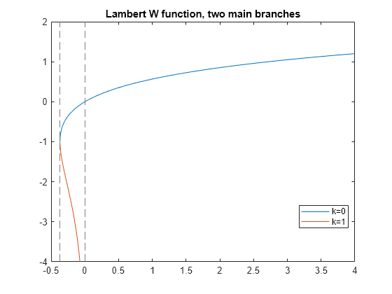
Plot the two main branches, and , of the Lambert W function.
syms x
fplot(lambertw(x))
hold on
fplot(lambertw(-1,x))
hold off
axis([-0.5 4 -4 2])
title('Lambert W function, two main branches')
legend('k=0','k=1','Location','best')
Lambert W Function Plot on Complex Plane
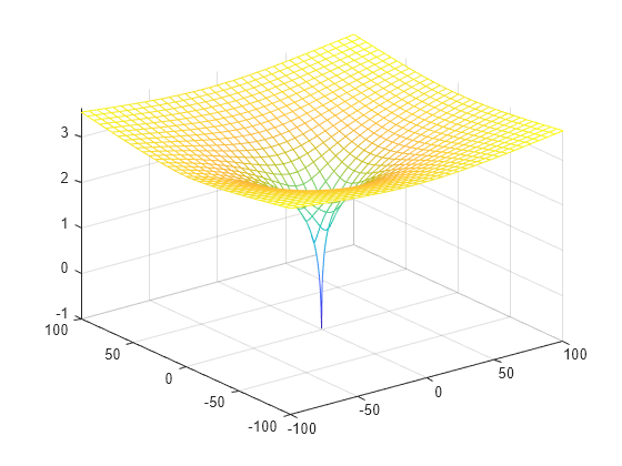
Plot the principal branch of the Lambert W function on the complex plane.
Plot the real value of the Lambert W function by using fmesh. Simultaneously plot the contours by setting 'ShowContours' to 'On'.
syms x y
f = lambertw(x + 1i*y);
interval = [-100 100 -100 100];
fmesh(real(f),interval,'ShowContours','On')
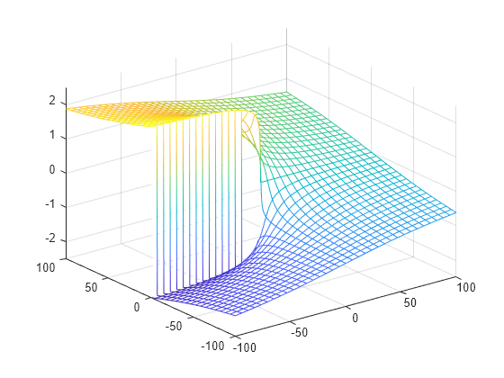
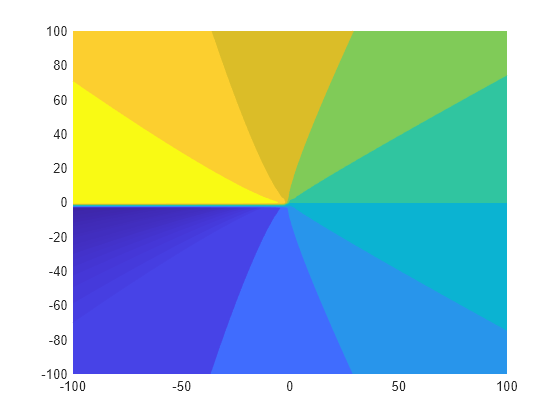
Plot the imaginary value of the Lambert W function. The plot has a branch cut along the negative real axis. Plot the contours separately.
fmesh(imag(f),interval)
fcontour(imag(f),interval,'Fill','on')
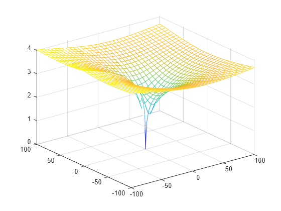
Plot the absolute value of the Lambert W function.
fmesh(abs(f),interval,'ShowContours','On')
Input Arguments
x — Input
number | vector | matrix | array | symbolic number | symbolic variable | symbolic array | symbolic function | symbolic expression
Input, specified as a number, vector, matrix, or array, or a symbolic number, variable, array, function, or expression.
At least one input argument must be a scalar, or both arguments must be vectors
or matrices of the same size. If one input argument is a scalar and the other is a
vector or matrix, lambertw expands the scalar into a vector or
matrix of the same size as the other argument with all elements equal to that
scalar.
k — Branch of Lambert W function
integer | vector or matrix of integers | symbolic integer | symbolic vector or matrix of integers
Branch of Lambert W function, specified as an integer, a vector or matrix of integers, a symbolic integer, or a symbolic vector or matrix of integers.
At least one input argument must be a scalar, or both arguments must be vectors
or matrices of the same size. If one input argument is a scalar and the other is a
vector or matrix, lambertw expands the scalar into a vector or
matrix of the same size as the other argument with all elements equal to that
scalar.
More About
Lambert W Function
The Lambert W function W(x) represents the solutions y of the equation for any complex number x.
For complex x, the equation has an infinite number of solutions y = lambertW(k,x) where k ranges over all integers.
For all real x ≥ 0, the equation has exactly one real solution y = lambertW(x) = lambertW(0,x).
For real x where , the equation has exactly two real solutions. The larger solution is represented by y = lambertW(x) and the smaller solution by y = lambertW(–1,x).
For , the equation has exactly one real solution y = –1 = lambertW(0, –exp(–1)) = lambertW(–1, -exp(–1)).
References
[1] Corless, R.M., G.H. Gonnet, D.E.G. Hare, D.J. Jeffrey, and D.E. Knuth. "On the Lambert W Function." Advances in Computational Mathematics, Vol. 5, pp. 329–359, 1996.
Version History
Introduced before R2006a
MATLAB Command
You clicked a link that corresponds to this MATLAB command:
Run the command by entering it in the MATLAB Command Window. Web browsers do not support MATLAB commands.

Select a Web Site
Choose a web site to get translated content where available and see local events and offers. Based on your location, we recommend that you select: .
You can also select a web site from the following list
How to Get Best Site Performance
Select the China site (in Chinese or English) for best site performance. Other bat365 country sites are not optimized for visits from your location.
Americas
- América Latina (Español)
- Canada (English)
- United States (English)
Europe
- Belgium (English)
- Denmark (English)
- Deutschland (Deutsch)
- España (Español)
- Finland (English)
- France (Français)
- Ireland (English)
- Italia (Italiano)
- Luxembourg (English)
- Netherlands (English)
- Norway (English)
- Österreich (Deutsch)
- Portugal (English)
- Sweden (English)
- Switzerland
- United Kingdom (English)
Asia Pacific
- Australia (English)
- India (English)
- New Zealand (English)
- 中国
- 日本Japanese (日本語)
- 한국Korean (한국어)