Data and Model for the Fit

We'll use data collected to study water pollution caused by industrial and domestic waste. These data are described in detail in Box, G.P., W.G. Hunter, and J.S. Hunter, Statistics for Experimenters (Wiley, 1978, pp. 483-487). The response variable is biochemical oxygen demand in mg/l, and the predictor variable is incubation time in days.

x = [1 2 3 5 7 10]';
y = [109 149 149 191 213 224]';

plot(x,y,'ko')
xlabel('Incubation (days), x') 
ylabel('Biochemical oxygen demand (mg/l), y')

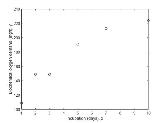
We'll assume that it is known that the first two observations were made with less precision than the remaining observations. They might, for example, have been made with a different instrument. Another common reason to weight data is that each recorded observation is actually the mean of several measurements taken at the same value of x. In the data here, suppose the first two values represent a single raw measurement, while the remaining four are each the mean of 5 raw measurements. Then it would be appropriate to weight by the number of measurements that went into each observation.

w = [1 1 5 5 5 5]';

Fit the Model without Weights

The model we'll fit to these data is a scaled exponential curve that becomes level as x becomes large.

modelFun = @(b,x) b(1).*(1-exp(-b(2).*x));

Just based on a rough visual fit, it appears that a curve drawn through the points might level out at a value of around 240 somewhere in the neighborhood of x = 15. So we'll use 240 as the starting value for b1, and since e^(-.5*15) is small compared to 1, we'll use .5 as the starting value for b2.

start = [240; .5];

The danger in ignoring measurement error is that the fit may be overly influenced by imprecise measurements, and may therefore not provide a good fit to measurements that are known precisely. Let's fit the data without weights and compare it to the points.

nlm = fitnlm(x,y,modelFun,start);
xx = linspace(0,12)';
line(xx,predict(nlm,xx),'linestyle','--','color','k')

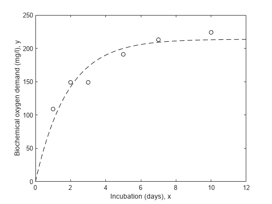
Notice that the fitted curve is pulled toward the first two points, but seems to miss the trend of the other points.

Fit the Model with Weights

Let's try repeating the fit using weights.

wnlm = fitnlm(x,y,modelFun,start,'Weight',w)

wnlm = 
Nonlinear regression model:
    y ~ b1*(1 - exp( - b2*x))

Estimated Coefficients:
          Estimate       SE       tStat       pValue  
          ________    ________    ______    __________

    b1     225.17         10.7    21.045    3.0134e-05
    b2    0.40078     0.064296    6.2333     0.0033745


Number of observations: 6, Error degrees of freedom: 4
Root Mean Squared Error: 24
R-Squared: 0.908,  Adjusted R-Squared 0.885
F-statistic vs. zero model: 696, p-value = 8.2e-06

line(xx,predict(wnlm,xx),'color','b')

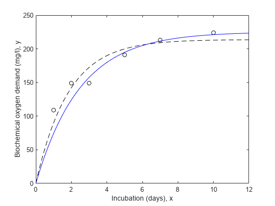
The estimated population standard deviation in this case describes the average variation for a "standard" observation with a weight, or measurement precision, of 1.

wnlm.RMSE

ans = 24.0096

An important part of any analysis is an estimate of the precision of the model fit. The coefficient display shows standard errors for the parameters, but we can also compute confidence intervals for them.

coefCI(wnlm)

ans = 2×2

  195.4650  254.8788
    0.2223    0.5793

Estimate the Response Curve

Next, we'll compute the fitted response values and confidence intervals for them. By default, those widths are for pointwise confidence bounds for the predicted value, but we will request simultaneous intervals for the entire curve.

[ypred,ypredci] = predict(wnlm,xx,'Simultaneous',true);
plot(x,y,'ko',xx,ypred,'b-',xx,ypredci,'r:')
xlabel('x') 
ylabel('y')
ylim([-150 350])
legend({'Data','Weighted fit','95% Confidence Limits'}, ...
    'location','SouthEast')

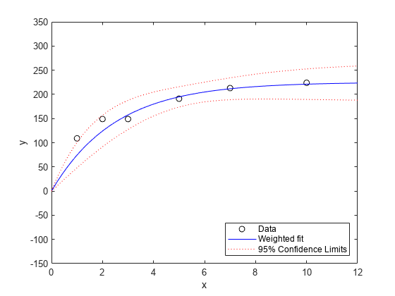
Notice that the two downweighted points are not fit as well by the curve as the remaining points. That's as you would expect for a weighted fit.

It's also possible to estimate prediction intervals for future observations at specified values of x. Those intervals will in effect assume a weight, or measurement precision, of 1.

[ypred,ypredci] = predict(wnlm,xx,'Simultaneous',true, ...
    'Prediction','observation');
plot(x,y,'ko',xx,ypred,'b-',xx,ypredci,'r:')
xlabel('x') 
ylabel('y')
ylim([-150 350])
legend({'Data','Weighted fit','95% Prediction Limits'}, ...
    'location','SouthEast')

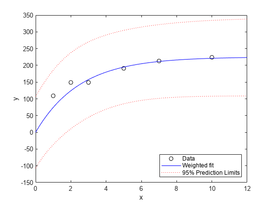
The absolute scale of the weights actually doesn't affect the parameter estimates. Rescaling the weights by any constant would have given us the same estimates. But they do affect the confidence bounds, since the bounds represent an observation with weight 1. Here you can see that the points with higher weight seem too close to the fitted line, compared with the confidence limits.

Suppose we are interested in a new observation that is based on the average of five measurements, just like the last four points in this plot. Specify observation weights by using the Weights name-value argument of the predict function.

[new_ypred,new_ypredci] = predict(wnlm,xx,'Simultaneous',true, ...
    'Prediction','observation','Weights',5*ones(size(xx)));
plot(x,y,'ko',xx,new_ypred,'b-',xx,new_ypredci,'r:')
xlabel('x') 
ylabel('y')
ylim([-150 350])
legend({'Data','Weighted fit','95% Prediction Limits'}, ...
    'location','SouthEast')

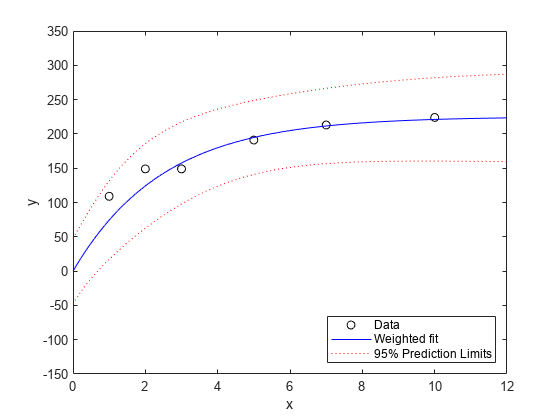
The predict function estimates the error variance at observation i by MSE*(1/W(i)), where MSE is the mean squared error. Therefore, the confidence intervals become narrow.

Residual Analysis

In addition to plotting the data and the fit, plot the residuals from a fit against the predictors, to diagnose any problems with the model. The residuals should appear independent and identically distributed (i.i.d.) but with a variance proportional to the inverse of the weights. Plot standardized residuals to confirm that the values are i.i.d. with the same variance. Standardized residuals are raw residuals divided by their estimated standard deviations.

r = wnlm.Residuals.Standardized;
plot(x,r,'b^')
xlabel('x')
ylabel('Standardized Residuals')

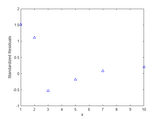
There is some evidence of systematic patterns in this residual plot. Notice how the last four residuals have a linear trend, suggesting that the model might not increase fast enough as x increases. Also, the magnitude of the residuals tends to decrease as x increases, suggesting that measurement error may depend on x. These deserve investigation, however, there are so few data points, that it's hard to attach significance to these apparent patterns.