bat365 Homepage

Stepwise Regression

Stepwise Regression to Select Appropriate Models

stepwiselm creates a linear model and automatically adds to or trims the model. To create a small model, start from a constant model. To create a large model, start with a model containing many terms. A large model usually has lower error as measured by the fit to the original data, but might not have any advantage in predicting new data.

stepwiselm can use all the name-value options from fitlm, with additional options relating to the starting and bounding models. In particular:

For a small model, start with the default lower bounding model: 'constant' (a model that has no predictor terms).
The default upper bounding model has linear terms and interaction terms (products of pairs of predictors). For an upper bounding model that also includes squared terms, set the Upper name-value pair to 'quadratic'.

Compare Large and Small Stepwise Models

Open Live Script

This example shows how to compare models that stepwiselm returns starting from a constant model and starting from a full interaction model.

Load the carbig data and create a table from some of the data.

load carbig
tbl = table(Acceleration,Displacement,Horsepower,Weight,MPG);

Create a mileage model stepwise starting from the constant model.

mdl1 = stepwiselm(tbl,'constant','ResponseVar','MPG')

1. Adding Weight, FStat = 888.8507, pValue = 2.9728e-103
2. Adding Horsepower, FStat = 3.8217, pValue = 0.00049608
3. Adding Horsepower:Weight, FStat = 64.8709, pValue = 9.93362e-15

mdl1 = 
Linear regression model:
    MPG ~ 1 + Horsepower*Weight

Estimated Coefficients:
                          Estimate         SE         tStat       pValue  
                         __________    __________    _______    __________

    (Intercept)              63.558        2.3429     27.127    1.2343e-91
    Horsepower             -0.25084      0.027279    -9.1952    2.3226e-18
    Weight                -0.010772    0.00077381    -13.921    5.1372e-36
    Horsepower:Weight    5.3554e-05    6.6491e-06     8.0542    9.9336e-15


Number of observations: 392, Error degrees of freedom: 388
Root Mean Squared Error: 3.93
R-squared: 0.748,  Adjusted R-Squared: 0.746
F-statistic vs. constant model: 385, p-value = 7.26e-116

Create a mileage model stepwise starting from the full interaction model.

mdl2 = stepwiselm(tbl,'interactions','ResponseVar','MPG')

1. Removing Acceleration:Displacement, FStat = 0.024186, pValue = 0.8765
2. Removing Displacement:Weight, FStat = 0.33103, pValue = 0.56539
3. Removing Acceleration:Horsepower, FStat = 1.7334, pValue = 0.18876
4. Removing Acceleration:Weight, FStat = 0.93269, pValue = 0.33477
5. Removing Horsepower:Weight, FStat = 0.64486, pValue = 0.42245

mdl2 = 
Linear regression model:
    MPG ~ 1 + Acceleration + Weight + Displacement*Horsepower

Estimated Coefficients:
                                Estimate         SE         tStat       pValue  
                               __________    __________    _______    __________

    (Intercept)                    61.285        2.8052     21.847    1.8593e-69
    Acceleration                 -0.34401       0.11862       -2.9     0.0039445
    Displacement                -0.081198      0.010071    -8.0623    9.5014e-15
    Horsepower                   -0.24313      0.026068    -9.3265    8.6556e-19
    Weight                     -0.0014367    0.00084041    -1.7095      0.088166
    Displacement:Horsepower    0.00054236    5.7987e-05     9.3531    7.0527e-19


Number of observations: 392, Error degrees of freedom: 386
Root Mean Squared Error: 3.84
R-squared: 0.761,  Adjusted R-Squared: 0.758
F-statistic vs. constant model: 246, p-value = 1.32e-117

Notice that:

mdl1 has four coefficients (the Estimate column), and mdl2 has six coefficients.
The adjusted R-squared of mdl1 is 0.746, which is slightly less (worse) than that of mdl2, 0.758.

Create a mileage model stepwise with a full quadratic model as the upper bound, starting from the full quadratic model:

mdl3 = stepwiselm(tbl,'quadratic','ResponseVar','MPG','Upper','quadratic');

1. Removing Acceleration:Horsepower, FStat = 0.075209, pValue = 0.78405
2. Removing Acceleration:Weight, FStat = 0.072756, pValue = 0.78751
3. Removing Horsepower:Weight, FStat = 0.12569, pValue = 0.72314
4. Removing Weight^2, FStat = 1.194, pValue = 0.27521
5. Removing Displacement:Weight, FStat = 1.2839, pValue = 0.25789
6. Removing Displacement^2, FStat = 2.069, pValue = 0.15114
7. Removing Horsepower^2, FStat = 0.74063, pValue = 0.39

Compare the three model complexities by examining their formulas.

mdl1.Formula

ans = 
MPG ~ 1 + Horsepower*Weight

mdl2.Formula

ans = 
MPG ~ 1 + Acceleration + Weight + Displacement*Horsepower

mdl3.Formula

ans = 
MPG ~ 1 + Weight + Acceleration*Displacement + Displacement*Horsepower + Acceleration^2

The adjusted $R^{2}$ values improve slightly as the models become more complex:

RSquared = [mdl1.Rsquared.Adjusted, ...
    mdl2.Rsquared.Adjusted, mdl3.Rsquared.Adjusted]

RSquared = 1×3

    0.7465    0.7580    0.7599

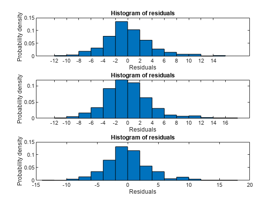
Compare residual plots of the three models.

subplot(3,1,1)
plotResiduals(mdl1)
subplot(3,1,2)
plotResiduals(mdl2)
subplot(3,1,3)
plotResiduals(mdl3)

The models have similar residuals. It is not clear which fits the data better.

Interestingly, the more complex models have larger maximum deviations of the residuals:

Rrange1 = [min(mdl1.Residuals.Raw),max(mdl1.Residuals.Raw)];
Rrange2 = [min(mdl2.Residuals.Raw),max(mdl2.Residuals.Raw)];
Rrange3 = [min(mdl3.Residuals.Raw),max(mdl3.Residuals.Raw)];
Rranges = [Rrange1;Rrange2;Rrange3]

Rranges = 3×2

  -10.7725   14.7314
  -11.4407   16.7562
  -12.2723   16.7927

Stepwise Regression

Stepwise Regression to Select Appropriate Models

Compare Large and Small Stepwise Models

See Also

Related Topics