Generalized Linear Models
What Are Generalized Linear Models?
Linear regression models describe a linear relationship between a response and one or more predictive terms. Many times, however, a nonlinear relationship exists. Nonlinear Regression describes general nonlinear models. A special class of nonlinear models, called generalized linear models, uses linear methods.
Recall that linear models have these characteristics:
At each set of values for the predictors, the response has a normal distribution with mean μ.
A coefficient vector b defines a linear combination Xb of the predictors X.
The model is μ = Xb.
In generalized linear models, these characteristics are generalized as follows:
At each set of values for the predictors, the response has a distribution that can be normal, binomial, Poisson, gamma, or inverse Gaussian, with parameters including a mean μ.
A coefficient vector b defines a linear combination Xb of the predictors X.
Prepare Data
To begin fitting a regression, put your data into a form that
fitting functions expect. All regression techniques begin with input
data in an array X and response data in a separate
vector y, or input data in a table or dataset array tbl and
response data as a column in tbl. Each row of the
input data represents one observation. Each column represents one
predictor (variable).
For a table or dataset array tbl, indicate
the response variable with the 'ResponseVar' name-value
pair:
mdl = fitglm(tbl,'ResponseVar','BloodPressure');
The response variable is the last column by default.
You can use numeric categorical predictors. A categorical predictor is one that takes values from a fixed set of possibilities.
For a numeric array
X, indicate the categorical predictors using the'Categorical'name-value pair. For example, to indicate that predictors2and3out of six are categorical:mdl = fitglm(X,y,'Categorical',[2,3]); % or equivalently mdl = fitglm(X,y,'Categorical',logical([0 1 1 0 0 0]));
For a table or dataset array
tbl, fitting functions assume that these data types are categorical:Logical vector
Categorical vector
Character array
String array
If you want to indicate that a numeric predictor is categorical, use the
'Categorical'name-value pair.
Represent missing numeric data as NaN. To
represent missing data for other data types, see Missing Group Values.
For a
'binomial'model with data matrixX, the responseycan be:Binary column vector — Each entry represents success (
1) or failure (0).Two-column matrix of integers — The first column is the number of successes in each observation, the second column is the number of trials in that observation.
For a
'binomial'model with table or datasettbl:Use the
ResponseVarname-value pair to specify the column oftblthat gives the number of successes in each observation.Use the
BinomialSizename-value pair to specify the column oftblthat gives the number of trials in each observation.
Dataset Array for Input and Response Data
For example, to create a dataset array from an Excel® spreadsheet:
ds = dataset('XLSFile','hospital.xls',...
    'ReadObsNames',true);
To create a dataset array from workspace variables:
load carsmall
ds = dataset(MPG,Weight);
ds.Year = ordinal(Model_Year);
Table for Input and Response Data
To create a table from workspace variables:
load carsmall
tbl = table(MPG,Weight);
tbl.Year = ordinal(Model_Year);
Numeric Matrix for Input Data, Numeric Vector for Response
For example, to create numeric arrays from workspace variables:
load carsmall
X = [Weight Horsepower Cylinders Model_Year];
y = MPG;
To create numeric arrays from an Excel spreadsheet:
[X, Xnames] = xlsread('hospital.xls');
y = X(:,4); % response y is systolic pressure
X(:,4) = []; % remove y from the X matrix
Notice that the nonnumeric entries, such as sex,
do not appear in X.
Choose Generalized Linear Model and Link Function
Often, your data suggests the distribution type of the generalized linear model.
| Response Data Type | Suggested Model Distribution Type |
|---|---|
| Any real number | 'normal' |
| Any positive number | 'gamma' or 'inverse gaussian' |
| Any nonnegative integer | 'poisson' |
Integer from 0 to n, where n is
a fixed positive value | 'binomial' |
Set the model distribution type with the Distribution name-value
pair. After selecting your model type, choose a link function to map
between the mean µ and the linear predictor Xb.
| Value | Description |
|---|---|
'comploglog' | log(–log((1 – µ))) = Xb |
| µ = Xb |
| log(µ) = Xb |
| log(µ/(1 – µ)) = Xb |
| log(–log(µ)) = Xb |
'probit' | Φ–1(µ) = Xb, where Φ is the normal (Gaussian) cumulative distribution function |
'reciprocal', default for the distribution 'gamma' | µ–1 = Xb |
| µp = Xb |
A cell array of the form | User-specified link function (see Custom Link Function) |
The nondefault link functions are mainly useful for binomial
models. These nondefault link functions are 'comploglog', 'loglog',
and 'probit'.
Custom Link Function
The link function defines the relationship f(µ)
= Xb between the mean response µ and
the linear combination Xb = X*b of
the predictors. You can choose one of the built-in link functions
or define your own by specifying the link function FL,
its derivative FD, and its inverse FI:
The link function
FLcalculates f(µ).The derivative of the link function
FDcalculates df(µ)/dµ.The inverse function
FIcalculates g(Xb) = µ.
You can specify a custom link function in either of two equivalent ways. Each way contains function handles that accept a single array of values representing µ or Xb, and returns an array the same size. The function handles are either in a cell array or a structure:
Cell array of the form
{FL FD FI}, containing three function handles, created using@, that define the link (FL), the derivative of the link (FD), and the inverse link (FI).Structure
s@:s.Links.Derivatives.Inverse
For example, to fit a model using the 'probit' link
function:
x = [2100 2300 2500 2700 2900 ...
     3100 3300 3500 3700 3900 4100 4300]';
n = [48 42 31 34 31 21 23 23 21 16 17 21]';
y = [1 2 0 3 8 8 14 17 19 15 17 21]';
g = fitglm(x,[y n],...
    'linear','distr','binomial','link','probit')
g =

Generalized Linear regression model:
    probit(y) ~ 1 + x1
    Distribution = Binomial

Estimated Coefficients:
                   Estimate     SE            tStat     pValue
    (Intercept)      -7.3628       0.66815    -11.02    3.0701e-28
    x1             0.0023039    0.00021352     10.79    3.8274e-27

12 observations, 10 error degrees of freedom
Dispersion: 1
Chi^2-statistic vs. constant model: 241, p-value = 2.25e-54
You can perform the same fit using a custom link function that
performs identically to the 'probit' link function:
s = {@norminv,@(x)1./normpdf(norminv(x)),@normcdf};
g = fitglm(x,[y n],...
    'linear','distr','binomial','link',s)
g =
Generalized Linear regression model:
link(y) ~ 1 + x1
Distribution = Binomial
Estimated Coefficients:
Estimate SE tStat pValue
(Intercept) -7.3628 0.66815 -11.02 3.0701e-28
x1 0.0023039 0.00021352 10.79 3.8274e-27
12 observations, 10 error degrees of freedom
Dispersion: 1
Chi^2-statistic vs. constant model: 241, p-value = 2.25e-54The two models are the same.
Equivalently, you can write s as a structure
instead of a cell array of function handles:
s.Link = @norminv; s.Derivative = @(x) 1./normpdf(norminv(x)); s.Inverse = @normcdf; g = fitglm(x,[y n],... 'linear','distr','binomial','link',s)
g =

Generalized Linear regression model:
    link(y) ~ 1 + x1
    Distribution = Binomial

Estimated Coefficients:
                   Estimate     SE            tStat     pValue
    (Intercept)      -7.3628       0.66815    -11.02    3.0701e-28
    x1             0.0023039    0.00021352     10.79    3.8274e-27

12 observations, 10 error degrees of freedom
Dispersion: 1
Chi^2-statistic vs. constant model: 241, p-value = 2.25e-54Choose Fitting Method and Model
There are two ways to create a fitted model.
Use
fitglmwhen you have a good idea of your generalized linear model, or when you want to adjust your model later to include or exclude certain terms.Use
stepwiseglmwhen you want to fit your model using stepwise regression.stepwiseglmstarts from one model, such as a constant, and adds or subtracts terms one at a time, choosing an optimal term each time in a greedy fashion, until it cannot improve further. Use stepwise fitting to find a good model, one that has only relevant terms.The result depends on the starting model. Usually, starting with a constant model leads to a small model. Starting with more terms can lead to a more complex model, but one that has lower mean squared error.
In either case, provide a model to the fitting function (which
is the starting model for stepwiseglm).
Specify a model using one of these methods.
Brief Model Name
| Name | Model Type |
|---|---|
'constant' | Model contains only a constant (intercept) term. |
'linear' | Model contains an intercept and linear terms for each predictor. |
'interactions' | Model contains an intercept, linear terms, and all products of pairs of distinct predictors (no squared terms). |
'purequadratic' | Model contains an intercept, linear terms, and squared terms. |
'quadratic' | Model contains an intercept, linear terms, interactions, and squared terms. |
'poly | Model is a polynomial with all terms up to degree i in
the first predictor, degree j in the second
predictor, etc. Use numerals 0 through 9.
For example, 'poly2111' has a constant plus all
linear and product terms, and also contains terms with predictor 1
squared. |
Terms Matrix
A terms matrix T is a
t-by-(p + 1) matrix specifying terms in a model,
where t is the number of terms, p is the number of
predictor variables, and +1 accounts for the response variable. The value of
T(i,j) is the exponent of variable j in term
i.
For example, suppose that an input includes three predictor variables x1,
x2, and x3 and the response variable
y in the order x1, x2,
x3, and y. Each row of T
represents one term:
[0 0 0 0]— Constant term or intercept[0 1 0 0]—x2; equivalently,x1^0 * x2^1 * x3^0[1 0 1 0]—x1*x3[2 0 0 0]—x1^2[0 1 2 0]—x2*(x3^2)
The 0 at the end of each term represents the response variable. In
general, a column vector of zeros in a terms matrix represents the position of the response
variable. If you have the predictor and response variables in a matrix and column vector,
then you must include 0 for the response variable in the last column of
each row.
Formula
A formula for a model specification is a character vector or string scalar of the form
',y ~
terms'
yis the response name.termscontainsVariable names
+to include the next variable-to exclude the next variable:to define an interaction, a product of terms*to define an interaction and all lower-order terms^to raise the predictor to a power, exactly as in*repeated, so^includes lower order terms as well()to group terms
Tip
Formulas include a constant (intercept) term by default. To
exclude a constant term from the model, include -1 in
the formula.
Examples:
'y ~ x1 + x2 + x3' is a three-variable linear model with
intercept.
'y ~ x1 + x2 + x3 - 1' is a
three-variable linear model without intercept.
'y ~ x1 + x2 +
                x3 + x2^2'
is a three-variable model with intercept and a
x2^2 term.
'y ~ x1 + x2^2 +
                x3'
is the same as the previous example, since x2^2
includes a x2 term.
'y ~ x1 + x2 + x3 +
                x1:x2'
includes an x1*x2
term.
'y ~ x1*x2 + x3' is the same as the
previous example, since x1*x2 = x1 + x2 +
x1:x2.
'y ~ x1*x2*x3 - x1:x2:x3' has
all interactions among x1, x2, and
x3, except the three-way
interaction.
'y ~ x1*(x2 + x3 + x4)' has all
linear terms, plus products of x1 with each of the other
variables.
Fit Model to Data
Create a fitted model using fitglm or stepwiseglm. Choose between them as in Choose Fitting Method and Model. For generalized
linear models other than those with a normal distribution, give a Distribution name-value
pair as in Choose Generalized Linear Model and Link Function. For
example,
mdl = fitglm(X,y,'linear','Distribution','poisson')
% or
mdl = fitglm(X,y,'quadratic',...
         'Distribution','binomial')
Examine Quality and Adjust the Fitted Model
After fitting a model, examine the result.
Model Display
A linear regression model shows several diagnostics when you enter its name or enter
disp(mdl). This display gives some of the basic
information to check whether the fitted model represents the data
adequately.
For example, fit a Poisson model to data constructed with two out of five predictors not affecting the response, and with no intercept term:
rng('default') % for reproducibility
X = randn(100,5);
mu = exp(X(:,[1 4 5])*[.4;.2;.3]);
y = poissrnd(mu);
mdl = fitglm(X,y,...
    'linear','Distribution','poisson')
mdl =


Generalized Linear regression model:
    log(y) ~ 1 + x1 + x2 + x3 + x4 + x5
    Distribution = Poisson

Estimated Coefficients:
                   Estimate     SE          tStat       pValue
    (Intercept)     0.039829     0.10793     0.36901       0.71212
    x1               0.38551    0.076116      5.0647    4.0895e-07
    x2             -0.034905    0.086685    -0.40266        0.6872
    x3              -0.17826    0.093552     -1.9054      0.056722
    x4               0.21929     0.09357      2.3436      0.019097
    x5               0.28918      0.1094      2.6432     0.0082126


100 observations, 94 error degrees of freedom
Dispersion: 1
Chi^2-statistic vs. constant model: 44.9, p-value = 1.55e-08
Notice that:
The display contains the estimated values of each coefficient in the
Estimatecolumn. These values are reasonably near the true values[0;.4;0;0;.2;.3], except possibly the coefficient ofx3is not terribly near0.There is a standard error column for the coefficient estimates.
The reported
pValue(which are derived from the t statistics under the assumption of normal errors) for predictors 1, 4, and 5 are small. These are the three predictors that were used to create the response datay.The
pValuefor(Intercept),x2andx3are larger than 0.01. These three predictors were not used to create the response datay. ThepValueforx3is just over.05, so might be regarded as possibly significant.The display contains the Chi-square statistic.
Diagnostic Plots
Diagnostic plots help you identify outliers, and see other problems in your model or fit. To illustrate these plots, consider binomial regression with a logistic link function.
The logistic model is useful for proportion data. It defines the relationship between the proportion p and the weight w by:
log[p/(1 – p)] = b1 + b2w
This example fits a binomial model to data. The data are derived
from carbig.mat, which contains measurements of
large cars of various weights. Each weight in w has
a corresponding number of cars in total and a corresponding
number of poor-mileage cars in poor.
It is reasonable to assume that the values of poor follow binomial distributions,
with the number of trials given by total and the
percentage of successes depending on w. This distribution
can be accounted for in the context of a logistic model by using a
generalized linear model with link function log(µ/(1
– µ)) = Xb.
This link function is called 'logit'.
w = [2100 2300 2500 2700 2900 3100 ...
     3300 3500 3700 3900 4100 4300]';
total = [48 42 31 34 31 21 23 23 21 16 17 21]';
poor = [1 2 0 3 8 8 14 17 19 15 17 21]';
mdl = fitglm(w,[poor total],...
    'linear','Distribution','binomial','link','logit')
mdl =

Generalized Linear regression model:
    logit(y) ~ 1 + x1
    Distribution = Binomial

Estimated Coefficients:
                   Estimate     SE            tStat      pValue
    (Intercept)       -13.38         1.394    -9.5986    8.1019e-22
    x1             0.0041812    0.00044258     9.4474    3.4739e-21

12 observations, 10 error degrees of freedom
Dispersion: 1
Chi^2-statistic vs. constant model: 242, p-value = 1.3e-54
See how well the model fits the data.
plotSlice(mdl)
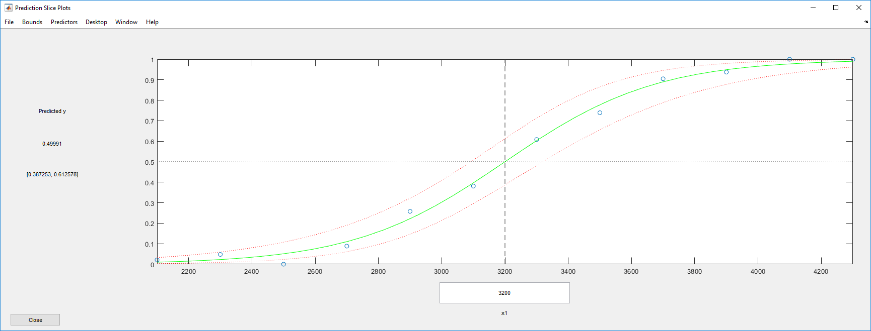
The fit looks reasonably good, with fairly wide confidence bounds.
To examine further details, create a leverage plot.
plotDiagnostics(mdl)
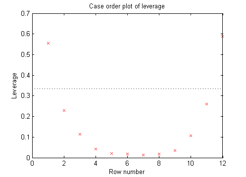
This is typical of a regression with points ordered by the predictor variable. The leverage of each point on the fit is higher for points with relatively extreme predictor values (in either direction) and low for points with average predictor values. In examples with multiple predictors and with points not ordered by predictor value, this plot can help you identify which observations have high leverage because they are outliers as measured by their predictor values.
Residuals — Model Quality for Training Data
There are several residual plots to help you discover errors, outliers, or correlations in the model or data. The simplest residual plots are the default histogram plot, which shows the range of the residuals and their frequencies, and the probability plot, which shows how the distribution of the residuals compares to a normal distribution with matched variance.
This example shows residual plots for a fitted Poisson model. The data construction has two out of five predictors not affecting the response, and no intercept term:
rng('default') % for reproducibility
X = randn(100,5);
mu = exp(X(:,[1 4 5])*[2;1;.5]);
y = poissrnd(mu);
mdl = fitglm(X,y,...
    'linear','Distribution','poisson');
Examine the residuals:
plotResiduals(mdl)
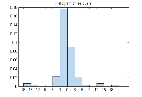
While most residuals cluster near 0, there are several near ±18. So examine a different residuals plot.
plotResiduals(mdl,'fitted')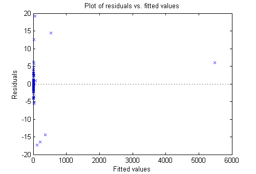
The large residuals don’t seem to have much to do with the sizes of the fitted values.
Perhaps a probability plot is more informative.
plotResiduals(mdl,'probability')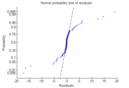
Now it is clear. The residuals do not follow a normal distribution. Instead, they have fatter tails, much as an underlying Poisson distribution.
Plots to Understand Predictor Effects and How to Modify a Model
This example shows how to understand the effect each predictor has on a regression model, and how to modify the model to remove unnecessary terms.
Create a model from some predictors in artificial data. The data do not use the second and third columns in
X. So you expect the model not to show much dependence on those predictors.rng('default') % for reproducibility X = randn(100,5); mu = exp(X(:,[1 4 5])*[2;1;.5]); y = poissrnd(mu); mdl = fitglm(X,y,... 'linear','Distribution','poisson');
Examine a slice plot of the responses. This displays the effect of each predictor separately.
plotSlice(mdl)
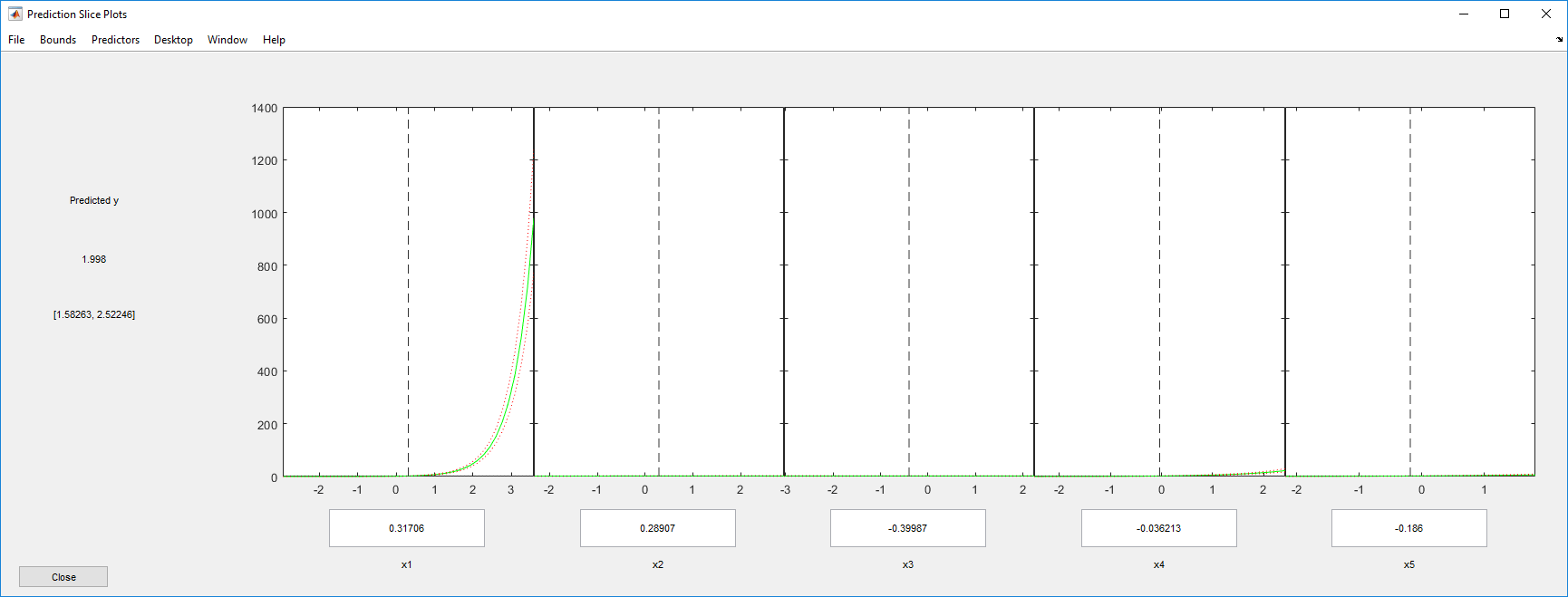
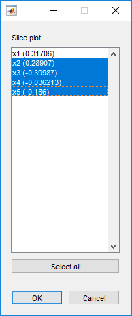
The scale of the first predictor is overwhelming the plot. Disable it using the Predictors menu.

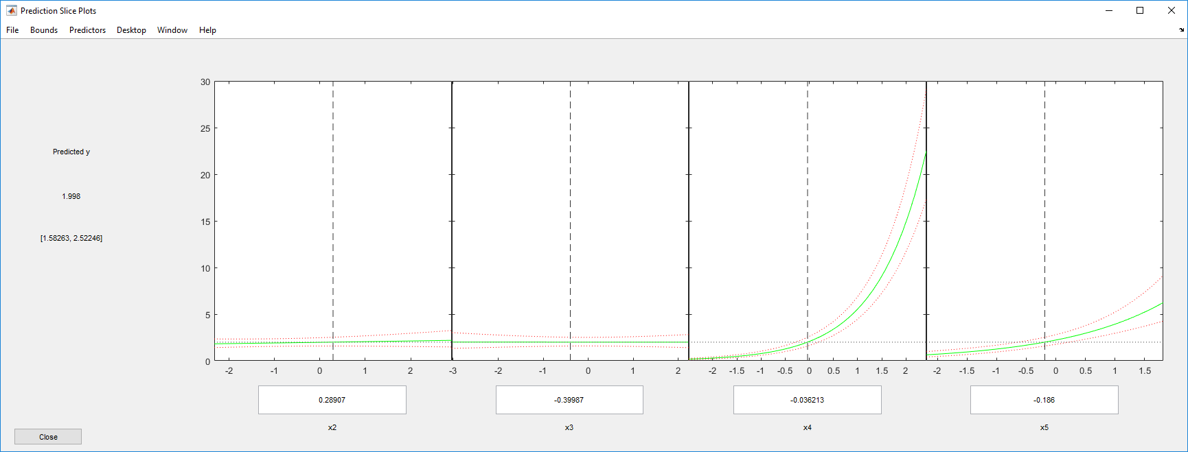
Now it is clear that predictors 2 and 3 have little to no effect.
You can drag the individual predictor values, which are represented by dashed blue vertical lines. You can also choose between simultaneous and non-simultaneous confidence bounds, which are represented by dashed red curves. Dragging the predictor lines confirms that predictors 2 and 3 have little to no effect.
Remove the unnecessary predictors using either
removeTermsorstep. Usingstepcan be safer, in case there is an unexpected importance to a term that becomes apparent after removing another term. However, sometimesremoveTermscan be effective whenstepdoes not proceed. In this case, the two give identical results.mdl1 = removeTerms(mdl,'x2 + x3')mdl1 = Generalized Linear regression model: log(y) ~ 1 + x1 + x4 + x5 Distribution = Poisson Estimated Coefficients: Estimate SE tStat pValue (Intercept) 0.17604 0.062215 2.8295 0.004662 x1 1.9122 0.024638 77.614 0 x4 0.98521 0.026393 37.328 5.6696e-305 x5 0.61321 0.038435 15.955 2.6473e-57 100 observations, 96 error degrees of freedom Dispersion: 1 Chi^2-statistic vs. constant model: 4.97e+04, p-value = 0mdl1 = step(mdl,'NSteps',5,'Upper','linear')
1. Removing x3, Deviance = 93.856, Chi2Stat = 0.00075551, PValue = 0.97807
2. Removing x2, Deviance = 96.333, Chi2Stat = 2.4769, PValue = 0.11553

mdl1 =


Generalized Linear regression model:
    log(y) ~ 1 + x1 + x4 + x5
    Distribution = Poisson

Estimated Coefficients:
                   Estimate    SE          tStat     pValue
    (Intercept)    0.17604     0.062215    2.8295       0.004662
    x1              1.9122     0.024638    77.614              0
    x4             0.98521     0.026393    37.328    5.6696e-305
    x5             0.61321     0.038435    15.955     2.6473e-57


100 observations, 96 error degrees of freedom
Dispersion: 1
Chi^2-statistic vs. constant model: 4.97e+04, p-value = 0
Predict or Simulate Responses to New Data
There are three ways to use a linear model to predict the response to new data:
predict
The predict method gives a prediction of
the mean responses and, if requested, confidence bounds.
This example shows how to predict and obtain confidence intervals on the
predictions using the predict method.
Create a model from some predictors in artificial data. The data do not use the second and third columns in
X. So you expect the model not to show much dependence on these predictors. Construct the model stepwise to include the relevant predictors automatically.rng('default') % for reproducibility X = randn(100,5); mu = exp(X(:,[1 4 5])*[2;1;.5]); y = poissrnd(mu); mdl = stepwiseglm(X,y,... 'constant','upper','linear','Distribution','poisson');
1. Adding x1, Deviance = 2515.02869, Chi2Stat = 47242.9622, PValue = 0
2. Adding x4, Deviance = 328.39679, Chi2Stat = 2186.6319, PValue = 0
3. Adding x5, Deviance = 96.3326, Chi2Stat = 232.0642, PValue = 2.114384e-52
Generate some new data, and evaluate the predictions from the data.
Xnew = randn(3,5) + repmat([1 2 3 4 5],[3,1]); % new data
[ynew,ynewci] = predict(mdl,Xnew)
ynew = 1.0e+04 * 0.1130 1.7375 3.7471 ynewci = 1.0e+04 * 0.0821 0.1555 1.2167 2.4811 2.8419 4.9407
feval
When you construct a model from a table or dataset array, feval is often more convenient for
predicting mean responses than predict. However,
feval does not provide confidence bounds.
This example shows how to predict mean responses using the feval method.
Create a model from some predictors in artificial data. The data do not use the second and third columns in
X. So you expect the model not to show much dependence on these predictors. Construct the model stepwise to include the relevant predictors automatically.rng('default') % for reproducibility X = randn(100,5); mu = exp(X(:,[1 4 5])*[2;1;.5]); y = poissrnd(mu); X = array2table(X); % create data table y = array2table(y); tbl = [X y]; mdl = stepwiseglm(tbl,... 'constant','upper','linear','Distribution','poisson');
1. Adding x1, Deviance = 2515.02869, Chi2Stat = 47242.9622, PValue = 0
2. Adding x4, Deviance = 328.39679, Chi2Stat = 2186.6319, PValue = 0
3. Adding x5, Deviance = 96.3326, Chi2Stat = 232.0642, PValue = 2.114384e-52
Generate some new data, and evaluate the predictions from the data.
Xnew = randn(3,5) + repmat([1 2 3 4 5],[3,1]); % new data
ynew = feval(mdl,Xnew(:,1),Xnew(:,4),Xnew(:,5)) % only need predictors 1,4,5
ynew =

   1.0e+04 *

    0.1130
    1.7375
    3.7471
Equivalently,
ynew = feval(mdl,Xnew(:,[1 4 5])) % only need predictors 1,4,5ynew = 1.0e+04 * 0.1130 1.7375 3.7471
random
The random method generates new random
response values for specified predictor values. The distribution of the response
values is the distribution used in the model. random
calculates the mean of the distribution from the predictors, estimated
coefficients, and link function. For distributions such as normal, the model
also provides an estimate of the variance of the response. For the binomial and
Poisson distributions, the variance of the response is determined by the mean;
random does not use a separate “dispersion”
estimate.
This example shows how to simulate responses using the random method.
Create a model from some predictors in artificial data. The data do not use the second and third columns in
X. So you expect the model not to show much dependence on these predictors. Construct the model stepwise to include the relevant predictors automatically.rng('default') % for reproducibility X = randn(100,5); mu = exp(X(:,[1 4 5])*[2;1;.5]); y = poissrnd(mu); mdl = stepwiseglm(X,y,... 'constant','upper','linear','Distribution','poisson');
1. Adding x1, Deviance = 2515.02869, Chi2Stat = 47242.9622, PValue = 0
2. Adding x4, Deviance = 328.39679, Chi2Stat = 2186.6319, PValue = 0
3. Adding x5, Deviance = 96.3326, Chi2Stat = 232.0642, PValue = 2.114384e-52
Generate some new data, and evaluate the predictions from the data.
Xnew = randn(3,5) + repmat([1 2 3 4 5],[3,1]); % new data
ysim = random(mdl,Xnew)
ysim = 1111 17121 37457The predictions from
randomare Poisson samples, so are integers.Evaluate the
randommethod again, the result changes.ysim = random(mdl,Xnew)
ysim =

        1175
       17320
       37126
Share Fitted Models
The model display contains enough information to enable someone else to recreate the model in a theoretical sense. For example,
rng('default') % for reproducibility
X = randn(100,5);
mu = exp(X(:,[1 4 5])*[2;1;.5]);
y = poissrnd(mu);
mdl = stepwiseglm(X,y,...
    'constant','upper','linear','Distribution','poisson')
1. Adding x1, Deviance = 2515.02869, Chi2Stat = 47242.9622, PValue = 0
2. Adding x4, Deviance = 328.39679, Chi2Stat = 2186.6319, PValue = 0
3. Adding x5, Deviance = 96.3326, Chi2Stat = 232.0642, PValue = 2.114384e-52

mdl =


Generalized Linear regression model:
    log(y) ~ 1 + x1 + x4 + x5
    Distribution = Poisson

Estimated Coefficients:
                   Estimate    SE          tStat     pValue
    (Intercept)    0.17604     0.062215    2.8295       0.004662
    x1              1.9122     0.024638    77.614              0
    x4             0.98521     0.026393    37.328    5.6696e-305
    x5             0.61321     0.038435    15.955     2.6473e-57


100 observations, 96 error degrees of freedom
Dispersion: 1
Chi^2-statistic vs. constant model: 4.97e+04, p-value = 0
You can access the model description programmatically, too. For example,
mdl.Coefficients.Estimate
ans =

    0.1760
    1.9122
    0.9852
    0.6132
mdl.Formula
ans =

log(y) ~ 1 + x1 + x4 + x5
References
[1] Collett, D. Modeling Binary Data. New York: Chapman & Hall, 2002.
[2] Dobson, A. J. An Introduction to Generalized Linear Models. New York: Chapman & Hall, 1990.
[3] McCullagh, P., and J. A. Nelder. Generalized Linear Models. New York: Chapman & Hall, 1990.
[4] Neter, J., M. H. Kutner, C. J. Nachtsheim, and W. Wasserman. Applied Linear Statistical Models, Fourth Edition. Irwin, Chicago, 1996.
