Choose Between Curve Fitting and Distribution Fitting

Curve fitting and distribution fitting are different types of data analysis.

Curve Fitting

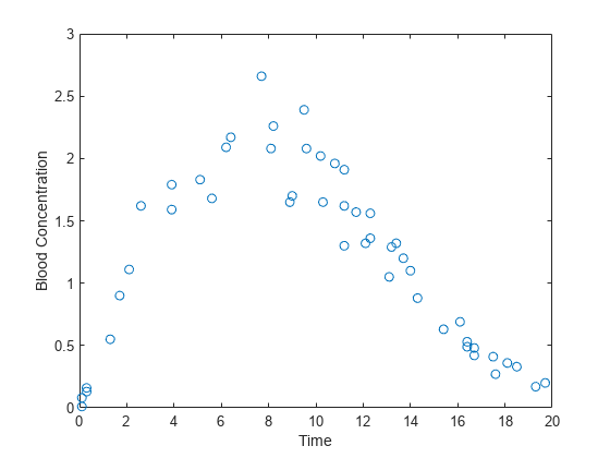
In the following experimental data, the predictor variable is time, the time after the ingestion of a drug. The response variable is conc, the concentration of the drug in the bloodstream. Assume that only the response data conc is affected by experimental error.

time = [ 0.1   0.1   0.3   0.3   1.3   1.7   2.1   2.6   3.9   3.9 ...
         5.1   5.6   6.2   6.4   7.7   8.1   8.2   8.9   9.0   9.5 ...
         9.6  10.2  10.3  10.8  11.2  11.2  11.2  11.7  12.1  12.3 ...
        12.3  13.1  13.2  13.4  13.7  14.0  14.3  15.4  16.1  16.1 ...
        16.4  16.4  16.7  16.7  17.5  17.6  18.1  18.5  19.3  19.7]';
conc = [0.01  0.08  0.13  0.16  0.55  0.90  1.11  1.62  1.79  1.59 ...
        1.83  1.68  2.09  2.17  2.66  2.08  2.26  1.65  1.70  2.39 ...
        2.08  2.02  1.65  1.96  1.91  1.30  1.62  1.57  1.32  1.56 ...
        1.36  1.05  1.29  1.32  1.20  1.10  0.88  0.63  0.69  0.69 ...
        0.49  0.53  0.42  0.48  0.41  0.27  0.36  0.33  0.17  0.20]';

Suppose you want to model blood concentration as a function of time. Plot conc against time.

plot(time,conc,'o');
xlabel('Time');
ylabel('Blood Concentration');

Assume that conc follows a two-parameter Weibull curve as a function of time. A Weibull curve has the form and parameters

where $$a$$ is a horizontal scaling, $$b$$ is a shape parameter, and $$c$$ is a vertical scaling.

Fit the Weibull model using nonlinear least squares.

modelFun =  @(p,x) p(3) .* (x./p(1)).^(p(2)-1) .* exp(-(x./p(1)).^p(2));
startingVals = [10 2 5];
nlModel = fitnlm(time,conc,modelFun,startingVals);

Plot the Weibull curve onto the data.

xgrid = linspace(0,20,100)';
line(xgrid,predict(nlModel,xgrid),'Color','r');

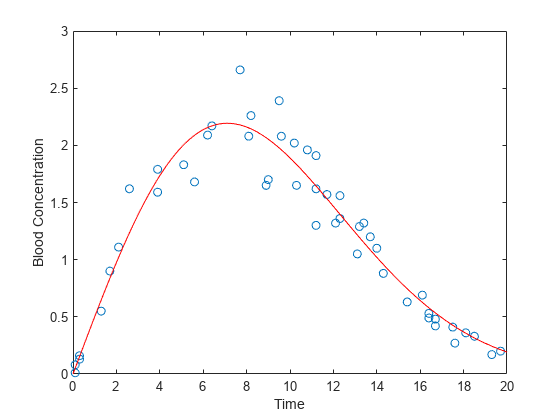
The fitted Weibull model is problematic. fitnlm assumes the experimental errors are additive and come from a symmetric distribution with constant variance. However, the scatter plot shows that the error variance is proportional to the height of the curve. Furthermore, the additive, symmetric errors imply that a negative blood concentration measurement is possible.

A more realistic assumption is that multiplicative errors are symmetric on the log scale. Under that assumption, fit a Weibull curve to the data by taking the log of both sides. Use nonlinear least squares to fit the curve:

nlModel2 = fitnlm(time,log(conc),@(p,x) log(modelFun(p,x)),startingVals);

Add the new curve to the existing plot.

line(xgrid,exp(predict(nlModel2,xgrid)),'Color',[0 .5 0],'LineStyle','--');
legend({'Raw Data','Additive Errors Model','Multiplicative Errors Model'});

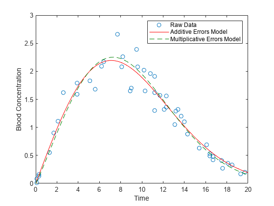
The model object nlModel2 contains estimates of precision. A best practice is to check the model's goodness of fit. For example, make residual plots on the log scale to check the assumption of constant variance for the multiplicative errors.

In this example, using the multiplicative errors model has little effect on the model predictions. For an example where the type of model has more of an impact, see Pitfalls in Fitting Nonlinear Models by Transforming to Linearity.

Functions for Curve Fitting

Distribution Fitting

Suppose you want to model the distribution of electrical component lifetimes. The variable life measures the time to failure for 50 identical electrical components.

life = [ 6.2 16.1 16.3 19.0 12.2  8.1  8.8  5.9  7.3  8.2 ...
        16.1 12.8  9.8 11.3  5.1 10.8  6.7  1.2  8.3  2.3 ...
         4.3  2.9 14.8  4.6  3.1 13.6 14.5  5.2  5.7  6.5 ...
         5.3  6.4  3.5 11.4  9.3 12.4 18.3 15.9  4.0 10.4 ...
         8.7  3.0 12.1  3.9  6.5  3.4  8.5  0.9  9.9  7.9]';

Visualize the data with a histogram.

binWidth = 2;
lastVal = ceil(max(life));
binEdges = 0:binWidth:lastVal+1;
h = histogram(life,binEdges);
xlabel('Time to Failure');
ylabel('Frequency');
ylim([0 10]);

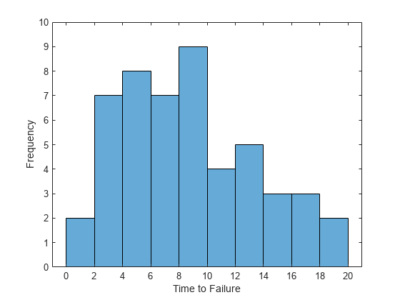
Because lifetime data often follows a Weibull distribution, one approach might be to use the Weibull curve from the previous curve fitting example to fit the histogram. To try this approach, convert the histogram to a set of points (x,y), where x is a bin center and y is a bin height, and then fit a curve to those points.

counts = histcounts(life,binEdges);
binCtrs = binEdges(1:end-1) + binWidth/2;
h.FaceColor = [.9 .9 .9];
hold on
plot(binCtrs,counts,'o');
hold off

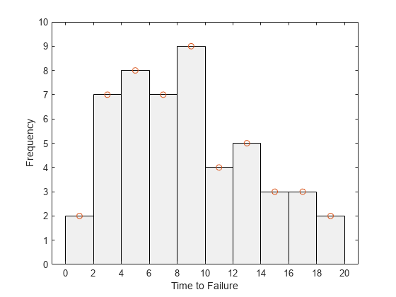
Fitting a curve to a histogram, however, is problematic and usually not recommended.

For many parametric distributions, maximum likelihood is a better way to estimate parameters because it avoids these problems. The Weibull pdf has almost the same form as the Weibull curve:

However, $$b/a$$ replaces the scale parameter $$c$$ because the function must integrate to 1. To fit a Weibull distribution to the data using maximum likelihood, use fitdist and specify 'Weibull' as the distribution name. Unlike least squares, maximum likelihood finds a Weibull pdf that best matches the scaled histogram without minimizing the sum of the squared differences between the pdf and the bar heights.

pd = fitdist(life,'Weibull');

Plot a scaled histogram of the data and superimpose the fitted pdf.

h = histogram(life,binEdges,'Normalization','pdf','FaceColor',[.9 .9 .9]);
xlabel('Time to Failure');
ylabel('Probability Density');
ylim([0 0.1]);
xgrid = linspace(0,20,100)';
pdfEst = pdf(pd,xgrid);
line(xgrid,pdfEst)

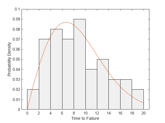
A best practice is to check the model's goodness of fit.

Although fitting a curve to a histogram is usually not recommended, the process is appropriate in some cases. For an example, see Fit Custom Distributions.

Functions for Distribution Fitting