Main Content

cmdscale

Classical multidimensional scaling

Syntax

Y = cmdscale(D)
[Y,e] = cmdscale(D)
[Y,e] = cmdscale(D,p)

Description

Y = cmdscale(D) takes an n-by-n distance matrix D, and returns an n-by-p configuration matrix Y. Rows of Y are the coordinates of n points in p-dimensional space for some p < n. When D is a Euclidean distance matrix, the distances between those points are given by D. p is the dimension of the smallest space in which the n points whose inter-point distances are given by D can be embedded.

[Y,e] = cmdscale(D) also returns the eigenvalues of Y*Y'. When D is Euclidean, the first p elements of e are positive, the rest zero. If the first k elements of e are much larger than the remaining (n-k), then you can use the first k columns of Y as k-dimensional points whose inter-point distances approximate D. This can provide a useful dimension reduction for visualization, e.g., for k = 2.

D need not be a Euclidean distance matrix. If it is non-Euclidean or a more general dissimilarity matrix, then some elements of e are negative, and cmdscale chooses p as the number of positive eigenvalues. In this case, the reduction to p or fewer dimensions provides a reasonable approximation to D only if the negative elements of e are small in magnitude.

[Y,e] = cmdscale(D,p) also accepts a positive integer p between 1 and n. p specifies the dimensionality of the desired embedding Y. If a p dimensional embedding is possible, then Y will be of size n-by-p and e will be of size p-by-1. If only a q dimensional embedding with q < p is possible, then Y will be of size n-by-q and e will be of size p-by-1. Specifying p may reduce the computational burden when n is very large.

You can specify D as either a full dissimilarity matrix, or in upper triangle vector form such as is output by pdist. A full dissimilarity matrix must be real and symmetric, and have zeros along the diagonal and positive elements everywhere else. A dissimilarity matrix in upper triangle form must have real, positive entries. You can also specify D as a full similarity matrix, with ones along the diagonal and all other elements less than one. cmdscale transforms a similarity matrix to a dissimilarity matrix in such a way that distances between the points returned in Y equal or approximate sqrt(1-D). To use a different transformation, you must transform the similarities prior to calling cmdscale.

Examples

collapse all

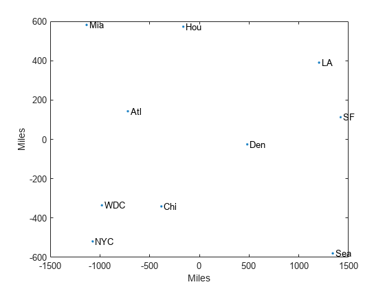
This example shows how to construct a map of 10 US cities based on the distances between those cities, using cmdscale.

First, create the distance matrix and pass it to cmdscale. In this example, D is a full distance matrix: it is square and symmetric, has positive entries off the diagonal, and has zeros on the diagonal.

cities = ...
{'Atl','Chi','Den','Hou','LA','Mia','NYC','SF','Sea','WDC'};
D = [    0  587 1212  701 1936  604  748 2139 2182   543;
       587    0  920  940 1745 1188  713 1858 1737   597;
      1212  920    0  879  831 1726 1631  949 1021  1494;
       701  940  879    0 1374  968 1420 1645 1891  1220;
      1936 1745  831 1374    0 2339 2451  347  959  2300;
       604 1188 1726  968 2339    0 1092 2594 2734   923;
       748  713 1631 1420 2451 1092    0 2571 2408   205;
      2139 1858  949 1645  347 2594 2571    0  678  2442;
      2182 1737 1021 1891  959 2734 2408  678    0  2329;
       543  597 1494 1220 2300  923  205 2442 2329     0];
[Y,eigvals] = cmdscale(D);

Next, look at the eigenvalues returned by cmdscale. Some of these are negative, indicating that the original distances are not Euclidean. This is because of the curvature of the earth.

format short g
[eigvals eigvals/max(abs(eigvals))]
ans = 10×2

   9.5821e+06            1
   1.6868e+06      0.17604
       8157.3    0.0008513
       1432.9   0.00014954
       508.67   5.3085e-05
       25.143    2.624e-06
   4.3252e-10   4.5138e-17
       -897.7  -9.3685e-05
      -5467.6   -0.0005706
       -35479   -0.0037026

However, in this case, the two largest positive eigenvalues are much larger in magnitude than the remaining eigenvalues. So, despite the negative eigenvalues, the first two coordinates of Y are sufficient for a reasonable reproduction of D.

Dtriu = D(find(tril(ones(10),-1)))';
maxrelerr = max(abs(Dtriu-pdist(Y(:,1:2))))./max(Dtriu)
maxrelerr = 
    0.0075371

Here is a plot of the reconstructed city locations as a map. The orientation of the reconstruction is arbitrary.

plot(Y(:,1),Y(:,2),'.')
text(Y(:,1)+25,Y(:,2),cities)
xlabel('Miles')
ylabel('Miles')

Figure contains an axes object. The axes object with xlabel Miles, ylabel Miles contains 11 objects of type line, text. One or more of the lines displays its values using only markers

Determine how the quality of reconstruction varies when you reduce points to distances using different metrics.

Generate ten points in 4-D space that are close to 3-D space. Take a linear transformation of the points so that their transformed values are close to a 3-D subspace that does not align with the coordinate axes.

rng default   % Set the seed for reproducibility
A = [normrnd(0,1,10,3) normrnd(0,0.1,10,1)];
B = randn(4,4);
X = A*B;

Reduce the points in X to distances by using the Euclidean metric. Find a configuration Y with the inter-point distances.

D = pdist(X,'euclidean');
Y = cmdscale(D);

Compare the quality of the reconstructions when using 2, 3, or 4 dimensions. The small maxerr3 value indicates that the first 3 dimensions provide a good reconstruction.

maxerr2 = max(abs(pdist(X)-pdist(Y(:,1:2)))) 
maxerr2 = 0.1631
maxerr3 = max(abs(pdist(X)-pdist(Y(:,1:3)))) 
maxerr3 = 0.0187
maxerr4 = max(abs(pdist(X)-pdist(Y)))
maxerr4 = 1.2546e-14

Reduce the points in X to distances by using the 'cityblock' metric. Find a configuration Y with the inter-point distances.

D = pdist(X,'cityblock');
[Y,e] = cmdscale(D);

Evaluate the quality of the reconstruction. e contains at least one negative element of large magnitude, which might account for the poor quality of the reconstruction.

maxerr = max(abs(pdist(X)-pdist(Y)))
maxerr = 9.0488
min(e)
ans = -5.6586

References

[1] Seber, G. A. F. Multivariate Observations. Hoboken, NJ: John Wiley & Sons, Inc., 1984.

Version History

Introduced before R2006a