bat365 Homepage

Assess Regression Neural Network Performance

Create a feedforward regression neural network model with fully connected layers using fitrnet. Use validation data for early stopping of the training process to prevent overfitting the model. Then, use the object functions of the model to assess its performance on test data.

Load Sample Data

Load the carbig data set, which contains measurements of cars made in the 1970s and early 1980s.

load carbig

Convert the Origin variable to a categorical variable. Then create a table containing the predictor variables Acceleration, Displacement, and so on, as well as the response variable MPG. Each row contains the measurements for a single car. Delete the rows of the table in which the table has missing values.

Origin = categorical(cellstr(Origin));
Tbl = table(Acceleration,Displacement,Horsepower, ...
    Model_Year,Origin,Weight,MPG);
Tbl = rmmissing(Tbl);

Partition Data

Split the data into training, validation, and test sets. First, reserve approximately one third of the observations for the test set. Then, split the remaining data in half to create the training and validation sets.

rng("default") % For reproducibility of the data partitions
cvp1 = cvpartition(size(Tbl,1),"Holdout",1/3);
testTbl = Tbl(test(cvp1),:);
remainingTbl = Tbl(training(cvp1),:);

cvp2 = cvpartition(size(remainingTbl,1),"Holdout",1/2);
validationTbl = remainingTbl(test(cvp2),:);
trainTbl = remainingTbl(training(cvp2),:);

Train Neural Network

Train a regression neural network model by using the training set. Specify the MPG column of tblTrain as the response variable, and standardize the numeric predictors. Evaluate the model at each iteration by using the validation set. Specify to display the training information at each iteration by using the Verbose name-value argument. By default, the training process ends early if the validation loss is greater than or equal to the minimum validation loss computed so far, six times in a row. To change the number of times the validation loss is allowed to be greater than or equal to the minimum, specify the ValidationPatience name-value argument.

Mdl = fitrnet(trainTbl,"MPG","Standardize",true, ...
    "ValidationData",validationTbl, ...
    "Verbose",1);

|==========================================================================================|
| Iteration  | Train Loss | Gradient   | Step       | Iteration  | Validation | Validation |
|            |            |            |            | Time (sec) | Loss       | Checks     |
|==========================================================================================|
|           1|  102.962345|   46.853164|    6.700877|    0.014315|  115.730384|           0|
|           2|   55.403995|   22.171181|    1.811805|    0.008511|   53.086379|           0|
|           3|   37.588848|   11.135231|    0.782861|    0.001906|   38.580002|           0|
|           4|   29.713458|    8.379231|    0.392009|    0.000483|   31.021379|           0|
|           5|   17.523851|    9.958164|    2.137584|    0.000488|   17.594863|           0|
|           6|   12.700624|    2.957771|    0.744551|    0.016949|   14.209019|           0|
|           7|   11.841152|    1.907378|    0.201770|    0.008734|   13.159899|           0|
|           8|   10.162988|    2.542555|    0.576907|    0.000714|   11.352490|           0|
|           9|    8.889095|    2.779980|    0.615716|    0.000493|   10.446334|           0|
|          10|    7.670335|    2.400272|    0.648711|    0.004829|   10.424337|           0|
|==========================================================================================|
| Iteration  | Train Loss | Gradient   | Step       | Iteration  | Validation | Validation |
|            |            |            |            | Time (sec) | Loss       | Checks     |
|==========================================================================================|
|          11|    7.416274|    0.505111|    0.214707|    0.001564|   10.522517|           1|
|          12|    7.338923|    0.880655|    0.119085|    0.002541|   10.648031|           2|
|          13|    7.149407|    1.784821|    0.277908|    0.000592|   10.800952|           3|
|          14|    6.866385|    1.904480|    0.472190|    0.000527|   10.839202|           4|
|          15|    6.815575|    3.339285|    0.943063|    0.000546|   10.031692|           0|
|          16|    6.428137|    0.684771|    0.133729|    0.000469|    9.867819|           0|
|          17|    6.363299|    0.456606|    0.125363|    0.001382|    9.720076|           0|
|          18|    6.289887|    0.742923|    0.152290|    0.000727|    9.576588|           0|
|          19|    6.215407|    0.964684|    0.183503|    0.000568|    9.422910|           0|
|          20|    6.078333|    2.124971|    0.566948|    0.000639|    9.599573|           1|
|==========================================================================================|
| Iteration  | Train Loss | Gradient   | Step       | Iteration  | Validation | Validation |
|            |            |            |            | Time (sec) | Loss       | Checks     |
|==========================================================================================|
|          21|    5.947923|    1.217291|    0.583867|    0.011433|    9.618400|           2|
|          22|    5.855505|    0.671774|    0.285123|    0.002249|    9.734680|           3|
|          23|    5.831802|    1.882061|    0.657368|    0.000519|   10.365968|           4|
|          24|    5.713261|    1.004072|    0.134719|    0.000455|   10.314258|           5|
|          25|    5.520766|    0.967032|    0.290156|    0.013475|   10.177322|           6|
|==========================================================================================|

Use the information inside the TrainingHistory property of the object Mdl to check the iteration that corresponds to the minimum validation mean squared error (MSE). The final returned model Mdl is the model trained at this iteration.

iteration = Mdl.TrainingHistory.Iteration;
valLosses = Mdl.TrainingHistory.ValidationLoss;
[~,minIdx] = min(valLosses);
iteration(minIdx)

ans = 19

Evaluate Test Set Performance

Evaluate the performance of the trained model Mdl on the test set testTbl by using the loss and predict object functions.

Compute the test set mean squared error (MSE). Smaller MSE values indicate better performance.

mse = loss(Mdl,testTbl,"MPG")

mse = 7.4101

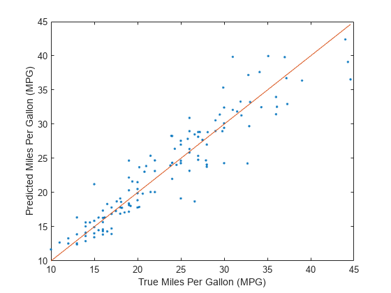
Compare the predicted test set response values to the true response values. Plot the predicted miles per gallon (MPG) along the vertical axis and the true MPG along the horizontal axis. Points on the reference line indicate correct predictions. A good model produces predictions that are scattered near the line.

predictedY = predict(Mdl,testTbl);

plot(testTbl.MPG,predictedY,".")
hold on
plot(testTbl.MPG,testTbl.MPG)
hold off
xlabel("True Miles Per Gallon (MPG)")
ylabel("Predicted Miles Per Gallon (MPG)")

Figure contains an axes object. The axes object with xlabel True Miles Per Gallon (MPG), ylabel Predicted Miles Per Gallon (MPG) contains 2 objects of type line. One or more of the lines displays its values using only markers

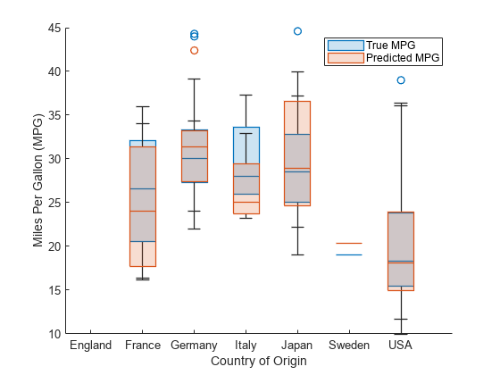
Use box plots to compare the distribution of predicted and true MPG values by country of origin. Create the box plots by using the boxchart function. Each box plot displays the median, the lower and upper quartiles, any outliers (computed using the interquartile range), and the minimum and maximum values that are not outliers. In particular, the line inside each box is the sample median, and the circular markers indicate outliers.

For each country of origin, compare the red box plot (showing the distribution of predicted MPG values) to the blue box plot (showing the distribution of true MPG values). Similar distributions for the predicted and true MPG values indicate good predictions.

boxchart(testTbl.Origin,testTbl.MPG)
hold on
boxchart(testTbl.Origin,predictedY)
hold off
legend(["True MPG","Predicted MPG"])
xlabel("Country of Origin")
ylabel("Miles Per Gallon (MPG)")

Figure contains an axes object. The axes object with xlabel Country of Origin, ylabel Miles Per Gallon (MPG) contains 2 objects of type boxchart. These objects represent True MPG, Predicted MPG.

For most countries, the predicted and true MPG values have similar distributions. Some discrepancies are possibly due to the small number of cars in the training and test sets.

Compare the range of MPG values for cars in the training and test sets.

trainSummary = grpstats(trainTbl(:,["MPG","Origin"]),"Origin", ...
    "range")

trainSummary=6×3 table
               Origin     GroupCount    range_MPG
               _______    __________    _________

    France     France          2           1.2   
    Germany    Germany        12          23.4   
    Italy      Italy           1             0   
    Japan      Japan          26          26.6   
    Sweden     Sweden          4             8   
    USA        USA            86            27

testSummary = grpstats(testTbl(:,["MPG","Origin"]),"Origin", ...
    "range")

testSummary=6×3 table
               Origin     GroupCount    range_MPG
               _______    __________    _________

    France     France          4          19.8   
    Germany    Germany        13          20.3   
    Italy      Italy           4          11.3   
    Japan      Japan          26          25.6   
    Sweden     Sweden          1             0   
    USA        USA            82            29

For countries like France, Italy, and Sweden, which have few cars in the training and test sets, the range of the MPG values varies significantly in both sets.

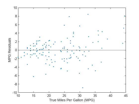
Plot the test set residuals. A good model usually has residuals scattered roughly symmetrically around 0. Clear patterns in the residuals are a sign that you can improve your model.

residuals = testTbl.MPG - predictedY;
plot(testTbl.MPG,residuals,".")
hold on
yline(0)
hold off
xlabel("True Miles Per Gallon (MPG)")
ylabel("MPG Residuals")

Figure contains an axes object. The axes object with xlabel True Miles Per Gallon (MPG), ylabel MPG Residuals contains 2 objects of type line, constantline. One or more of the lines displays its values using only markers

The plot suggests that the residuals are well distributed.

You can obtain more information about the observations with the greatest residuals, in terms of absolute value.

[~,residualIdx] = sort(residuals,"descend", ...
    "ComparisonMethod","abs");
residuals(residualIdx)

ans = 130×1

   -8.8469
    8.4427
    8.0493
    7.8996
   -6.2220
    5.8589
    5.7007
   -5.6733
   -5.4545
    5.1899
      ⋮

Display the three observations with the greatest residuals, that is, with magnitudes greater than 8.

testTbl(residualIdx(1:3),:)

ans=3×7 table
    Acceleration    Displacement    Horsepower    Model_Year    Origin    Weight    MPG 
    ____________    ____________    __________    __________    ______    ______    ____

        17.6             91             68            82        Japan      1970       31
        11.4            168            132            80        Japan      2910     32.7
        13.8             91             67            80        Japan      1850     44.6

Assess Regression Neural Network Performance

Load Sample Data

Partition Data

Train Neural Network

Evaluate Test Set Performance

See Also