Estimate Frequency Response Using Model Linearizer
This example shows how to estimate the frequency response of a portion of a Simulink® model using the Model Linearizer. To estimate the frequency response, you specify the portion of the model you want to estimate, the operating point for estimation, and the input signal to use for estimation.
Open Simulink Model and Model Linearizer
Open the Simulink model.
sys = 'scdDCMotor';
open_system(sys)
To open the Model Linearizer, in the Simulink model window, in the Apps gallery, click Model Linearizer.
Specify Portion of Model to Estimate
By default, Model Linearizer uses the linearization analysis points defined
in the model (the model I/Os) to determine where to inject the test
signal and where to measure the frequency response. The model
scdDCMotor contains predefined linear analysis points: an input point
at the compensator output, and an open-loop output after the unit gain block. For this
example, use these predefined model I/Os to obtain the frequency response of the inner
loop of the model with the outer loop open.
If you want to obtain the frequency response of a different portion of the model, on the Estimation tab of Model Linearizer, use the Analysis I/Os drop-down list. Analysis points for estimation work the same way as analysis points for linearization. For more information about linear analysis points, see Specify Portion of Model to Linearize.
Specify Operating Point for Estimation
You perform frequency response estimation at a steady-state operating point of the model. You can compute or specify an operating point in Model Linearizer using the Operating Point drop-down list. By default, Model Linearizer uses the operating point defined by the model initial conditions. For this example, use that operating point. For more information about operating points, see About Operating Points.
Create Input Signal for Estimation
Frequency response estimation injects an input signal into the input analysis point you specify for estimation. For this example, configure a sinestream signal, which is a series of sinusoidal perturbations at frequencies you specify. (For more information about input signals, see Estimation Input Signals.)
On the Estimation tab, in the Input Signal drop-down list, select
Sinestream. The Create sinestream input dialog box opens.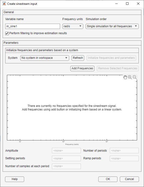
To specify frequency points for the input signal, click Add Frequencies. In the Add frequencies dialog box, specify the frequency range and number of points for the input signal. The frequency points you specify are the frequencies at which Model Linearizer computes the estimated response.
For this example, specify a range from 0.1 to 100 rad/s. Also, specify 100 logarithmically spaced frequencies.
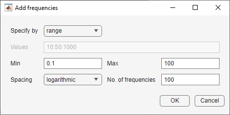
Click OK. The added points are visible in the frequency content viewer of the Create sinestream input dialog box.
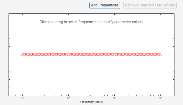
Select all these frequency points for the estimation input signal.
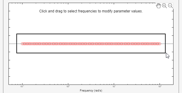
Specify the amplitude of the input signal. Enter
1in the Amplitude field. When you specify a scalar value, Model Linearizer uses the same amplitude for all frequencies.Click OK to create the sinestream input signal. The new input signal,
in_sine1, appears in the Linear Analysis Workspace.
Estimate Frequency Response
You can now estimate the frequency response and generate a frequency-domain plot of
the result. To do so, click ![]() Bode. The estimated frequency response, appears in the
Linear Analysis Workspace as the
Bode. The estimated frequency response, appears in the
Linear Analysis Workspace as the frd model
estsys1.
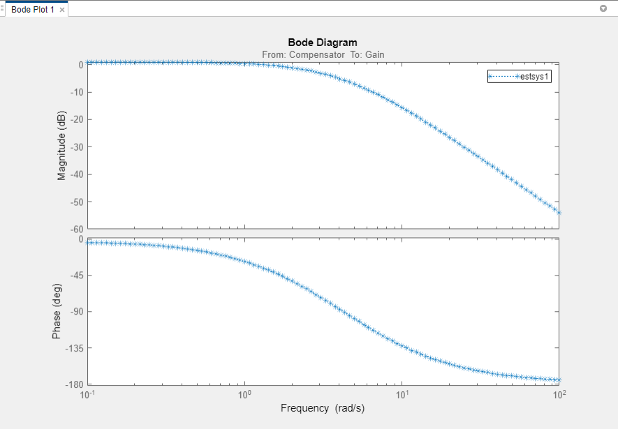
To export the estimated frequency response model to the MATLAB® workspace for further analysis, right click on the model in the Linear Analysis Workspace and select Export to MATLAB Workspace section.
Analyze Estimated Frequency Response
The simulation results viewer in Model Linearizer lets you examine further details of the frequency response estimation. For more information, see Analyze Estimated Frequency Response.
Related Topics
- Frequency Response Estimation Basics
- Estimation Input Signals
- Analyze Estimated Frequency Response
- Estimate Frequency Response at the Command Line
