A frequency response describes the steady-state response of a system to sinusoidal inputs of varying frequencies and lets control engineers analyze and design control systems in the frequency domain.
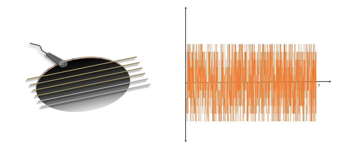
To understand why the frequency domain is important consider an acoustic guitar. If we place a microphone close to its soundboard and pluck one of the strings (Fig. 1. left), the vibrating string will resonate in the guitar cavity and produce a sound wave that is captured by the microphone. Looking at the time trace of the captured signal (Fig. 1, right) it is difficult to quickly extract information about what is going on.

Figure 1: The vibration resonates in the guitar cavity and produces a sound wave (left). Time trace of signal in the time domain (right).
When we look at that same signal in the frequency domain on a spectrum analyzer or by taking a fast Fourier transform (FFT) of the time domain signal, we see an amplitude peak at some frequency (Fig. 2, left). This peak frequency is the underlying tone that forms the note we just played. When we adjust the tuner knob or press the string to the neck of the guitar, we change the preload or the effective length of that string. This will shift the frequency at which the string resonates up or down, and we produce a different note (Fig. 2, right). With this simple analysis in the frequency domain, we can see how the guitar (the system) responds to plucking (the system input).

Figure 2: The same signal is shown in the frequency domain (left). Shifting the resonant frequency of the string by preloading it (right).
This analogy can be carried over to other systems where we are interested in the system’s response to inputs or stimuli from the environment. We can get insights into the system dynamics such as frequency of a resonant peak, DC gain, bandwidth, phase delay, and phase and gain margins for a closed-loop system.
Getting the Frequency Response of a System
The chart below helps identify an approach (shown in gray) to obtain the frequency response of a system using MATLAB® and Simulink®.
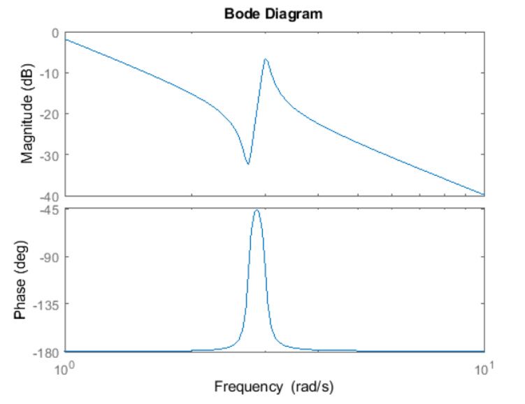
- If you have a linear representation of the system in the form of a transfer function or state-space model, you can plot the frequency response using one of the three plots: a Bode plot, Nyquist plot, or a Nichols chart. The Bode plot displays magnitude and phase as functions of the frequency of the excitation signal (Fig. 4).
For example, given the transfer function representation of a system \((H)\),
$$H(s) = {s^2+ 0.1s + 7.5\over s^4+0.12s^3+9s^2}.$$
you can plot its frequency response in MATLAB using the following commands:
\(H = {tf([1 \quad 0.1\quad 7.5], [1 \quad 0.12 \quad 9 \quad 0 \quad 0]});\)
\(bode(H)\)

Figure 4: Bode plot.
In some situations, a linear representation of the system might not be available.
- In that case, if you have access to input-output test data from the physical system, you can use data-driven modeling approaches with System Identification Toolbox™ to identify transfer function, state-space representations, and frequency response models of the system.
- If you use Simulink to model the system dynamics, you can use the Model Linearizer app in Simulink Control Design™ to linearize your model to create a linear state-space approximation of your Simulink model and plot the frequency response.
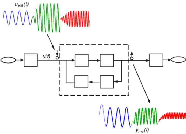
- In case the Simulink models cannot linearize due to discontinuities, you can use frequency response estimation to directly estimate a frequency response model.

Figure 5: Frequency response estimation in Simulink.
Simulink Control Design provides two approaches for estimating a frequency response model of your system.
Offline frequency response estimation
The Model Linearizer app excites the system with an input perturbation signal at specified frequencies and logs the response at the model output during simulation (Fig. 5). Post simulation, the logged input and output signals are processed to compute a frequency response of the model.
Online frequency response estimation
The frequency response of a physical plant is estimated during real-time operation with the Frequency Response Estimator block. This blocks injects sinusoidal test signals into the plant at the nominal operating point and the frequency response is continually refined as the output signal data is collected
The following table shows the perturbation signals that you can inject based on your estimation needs of frequency range, accuracy, and speed of estimation.
| Input signal type | Availability of offline/online estimation | Frequency range (narrowband/wideband) | Accuracy | Speed of estimation | Useful when… |
|---|---|---|---|---|---|
| Scale of 1 (low) to 5 (high) | |||||
| Sinestream | Offline, Online | Narrowband | ★★★★★ | ★ | System contains strong nonlinearities or you require highly accurate frequency response models. |
| Chirp | Offline | Wideband | ★★ | ★★★ | System is nearly linear in the frequency range. Also useful when you want to obtain a response quickly for a lot of frequency points. |
| PRBS | Offline | Wideband | ★★ | ★★★ | System contains high frequency switching components such as with communications and power electronics systems. |
| Step | Offline | Wideband | ★ | ★★★ | Exciting the system uniformly at all frequencies up to Nyquist frequency |
| Random | Offline | Wideband | ★★ | ★★★ | You don’t have much knowledge about the system you are estimating. |
In summary, computing a frequency response of a system is important for control analysis and design. MATLAB and Simulink provide different approaches you can use to get the frequency response of your system. To learn more about these approaches, see the examples and the references below.

