Main Content

fsst

Fourier synchrosqueezed transform

Description

s = fsst(x) returns the Fourier Synchrosqueezed Transform of the input signal, x. Each column of s contains the synchrosqueezed spectrum of a windowed segment of x.

example

[s,w,n] = fsst(x) returns a vector of normalized frequencies, w, and a vector of sample numbers, n, at which the Fourier synchrosqueezed transform is computed. w corresponds to the columns of s and n corresponds to the rows of s.

example

[s,f,t] = fsst(x,fs) returns a vector of cyclical frequencies, f, and a vector of time instants, t, expressed in terms of the sample rate, fs.

example

[s,f,t] = fsst(x,ts) specifies the sample time, ts, as a duration scalar. t is in the same units as ts. The units of f are reciprocal to the units of ts.

example

[___] = fsst(___,window) uses window to divide the signal into segments and perform windowing. You can use any combination of input arguments from previous syntaxes to obtain the corresponding output arguments.

fsst(___) with no output arguments plots the synchrosqueezed transform in the current figure window.

example

fsst(___,freqloc) specifies the axis on which to plot the frequency.

Examples

collapse all

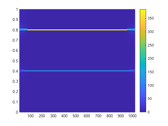
Generate 1024 samples of a signal that consists of a sum of sinusoids embedded in white Gaussian noise. The normalized frequencies of the sinusoids are 2π/5 rad/sample and 4π/5 rad/sample. The higher frequency sinusoid has 3 times the amplitude of the other sinusoid.

N = 1024;
n = 0:N-1;

w0 = 2*pi/5;
x = sin(w0*n)+3*sin(2*w0*n);

Compute the Fourier synchrosqueezed transform of the signal. Plot the result.

[s,w,n] = fsst(x);

mesh(n,w/pi,abs(s))

axis tight
view(2)
colorbar

Figure contains an axes object. The axes object contains an object of type surface.

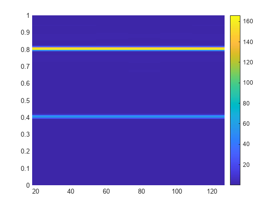
Compute the conventional short-time Fourier transform of the signal for comparison. Use the default values of spectrogram. Plot the result.

[s,w,n] = spectrogram(x);
 
surf(n,w/pi,abs(s),'EdgeColor','none')

axis tight
view(2)
colorbar

Figure contains an axes object. The axes object contains an object of type surface.

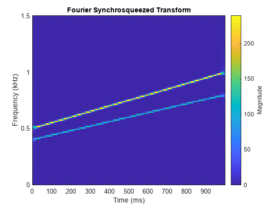
Generate a signal that consists of two chirps. The signal is sampled at 3 kHz for one second. The first chirp has an initial frequency of 400 Hz and reaches 800 Hz at the end of the sampling. The second chirp starts at 500 Hz and reaches 1000 Hz at the end. The second chirp has twice the amplitude of the first chirp.

fs = 3000;
t = 0:1/fs:1-1/fs;

x1 = chirp(t,400,t(end),800);
x2 = 2*chirp(t,500,t(end),1000);

Compute and plot the Fourier synchrosqueezed transform of the signal.

fsst(x1+x2,fs,'yaxis')

Figure contains an axes object. The axes object with title Fourier Synchrosqueezed Transform, xlabel Time (ms), ylabel Frequency (kHz) contains an object of type image.

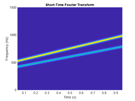
Compare the synchrosqueezed transform with the short-time Fourier transform (STFT). Compute the STFT using the spectrogram function. Specify the default parameters used by fsst:

  • A 256-point Kaiser window with β = 10 to window the signal

  • An overlap of 255 samples between adjoining windowed segments

  • An FFT length of 256

[stft,f,t] = spectrogram(x1+x2,kaiser(256,10),255,256,fs);

Plot the absolute value of the STFT.

mesh(t,f,abs(stft))

xlabel('Time (s)') 
ylabel('Frequency (Hz)')
title('Short-Time Fourier Transform')
axis tight
view(2)

Figure contains an axes object. The axes object with title Short-Time Fourier Transform, xlabel Time (s), ylabel Frequency (Hz) contains an object of type surface.

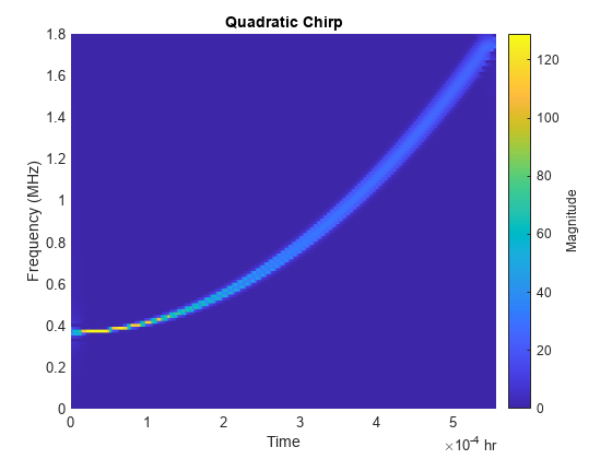
Compute and display the Fourier synchrosqueezed transform of a quadratic chirp that starts at 100 Hz and crosses 200 Hz at t = 1 s. Specify a sample rate of 1 kHz. Express the sample time as a duration scalar.

fs = 1000;
t = 0:1/fs:2;
ts = duration(0,0,1/fs);

x = chirp(t,100,1,200,'quadratic');

fsst(x,ts,'yaxis')

title('Quadratic Chirp')

Figure contains an axes object. The axes object with title Quadratic Chirp, xlabel Time, ylabel Frequency (MHz) contains an object of type surface.

The synchrosqueezing algorithm works under the assumption that the frequency of the signal varies slowly. Thus the spectrum is better concentrated at early times, where the rate of change of frequency is smaller.

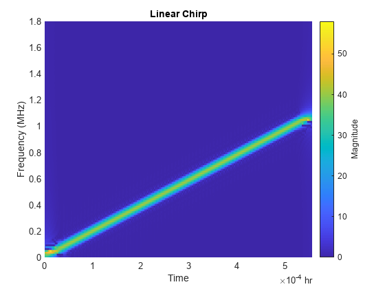
Compute and display the Fourier synchrosqueezed transform of a linear chirp that starts at DC and crosses 150 Hz at t = 1 s. Use a 256-sample Hamming window.

x = chirp(t,0,1,150);

fsst(x,ts,hamming(256),'yaxis')

title('Linear Chirp')

Figure contains an axes object. The axes object with title Linear Chirp, xlabel Time, ylabel Frequency (MHz) contains an object of type surface.

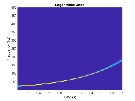
Compute and display the Fourier synchrosqueezed transform of a logarithmic chirp. The chirp is sampled at 1 kHz, starts at 20 Hz, and crosses 60 Hz at t = 1 s. Use a 256-sample Kaiser window with β = 20.

x = chirp(t,20,1,60,'logarithmic');

[s,f,t] = fsst(x,fs,kaiser(256,20));

clf
mesh(t,f,(abs(s)))

title('Logarithmic Chirp') 
xlabel('Time (s)')
ylabel('Frequency (Hz)')
view(2)

Figure contains an axes object. The axes object with title Logarithmic Chirp, xlabel Time (s), ylabel Frequency (Hz) contains an object of type surface.

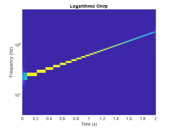
Use a logarithmic scale for the frequency axis. The transform becomes a straight line.

ax = gca;
ax.YScale = 'log';
axis tight

Figure contains an axes object. The axes object with title Logarithmic Chirp, xlabel Time (s), ylabel Frequency (Hz) contains an object of type surface.

This example shows that the Fourier Synchrosqueezed Transform, despite the sharp ridges it produces, cannot resolve arbitrarily spaced sinusoids. The width of the window used by the transform dictates how closely spaced two sinusoids can be and still be detected as distinct.

Consider a sinusoid, f(x)=ej2πνx, windowed with a Gaussian window, g(t)=e-πt2. The short-time transform is

Vgf(t,η)=ej2πνt-e-π(x-t)2e-j2π(x-t)(η-ν)dx=e-π(η-ν)2ej2πνt.

When viewed as a function of frequency, the transform combines a constant (in time) oscillation at ν with Gaussian decay away from it. The synchrosqueezing estimate of the instantaneous frequency,

Ωgf(t,η)=1j2πe-π(η-ν)2tej2πνte-π(η-ν)2ej2πνt=ν,

equals the value obtained by using the standard definition,

νinst=12πddtargf(t)=12πddt2πνt.

For a superposition of sinusoids,

f(x)=k=1KAkej2πνkx,

the short-time transform becomes

Vgf(t,η)=k=1KAke-π(η-νk)2ej2πνkt.

Create 1024 samples of a signal consisting of two sinusoids. One sinusoid has a normalized frequency of ω0=π/5 rad/sample. The other sinusoid has three times the frequency and three times the amplitude.

N = 1024;
n = 0:N-1;

w0 = pi/5;
x = exp(1j*w0*n)+3*exp(1j*3*w0*n);

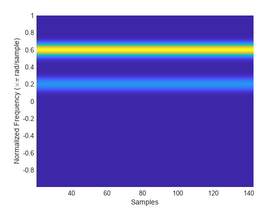
Use the spectrogram function to compute the short-time Fourier transform of the signal. Use a 256-sample Gaussian window with α=20, 255 samples of overlap between adjoining sections, and 1024 DFT points. Plot the absolute value of the transform.

Nw = 256;
nfft = 1024;
alpha = 20;

[s,w,t] = spectrogram(x,gausswin(Nw,alpha),Nw-1,nfft,"centered");

surf(t,w/pi,abs(s),EdgeColor="none")
view(2)
axis tight
xlabel("Samples")
ylabel("Normalized Frequency (\times\pi rad/sample)")

Figure contains an axes object. The axes object with xlabel Samples, ylabel Normalized Frequency ( times pi blank rad/sample) contains an object of type surface.

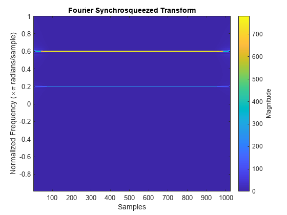
The Fourier synchrosqueezed transform, implemented in the fsst function, results in a sharper, better localized estimate of the spectrum.

[ss,sw,st] = fsst(x,[],gausswin(Nw,alpha));

fsst(x,"yaxis")

Figure contains an axes object. The axes object with title Fourier Synchrosqueezed Transform, xlabel Samples, ylabel Normalized Frequency ( times pi blank radians/sample) contains an object of type image.

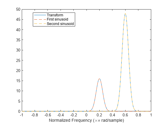
The sinusoids are visible as constant oscillations at the expected frequency values. To see that the decay away from the ridges is Gaussian, plot an instantaneous value of the transform and overlay two instances of a Gaussian. Express the Gaussian amplitude and standard deviation in terms of α and the window length. Recall that the standard deviation of the frequency-domain window is the reciprocal of the standard deviation of the time-domain window.

rstdev = (Nw-1)/(2*alpha);
amp = rstdev*sqrt(2*pi);

instransf = abs(s(:,128));

plot(w/pi,instransf)
hold on
plot(w/pi,[1 3]*amp.*exp(-rstdev^2/2*(w-[1 3]*w0).^2),"--")
hold off
xlabel("Normalized Frequency (\times\pi rad/sample)")
legend(["Transform" "First sinusoid" "Second sinusoid"],Location="best")

Figure contains an axes object. The axes object with xlabel Normalized Frequency ( times pi blank rad/sample) contains 3 objects of type line. These objects represent Transform, First sinusoid, Second sinusoid.

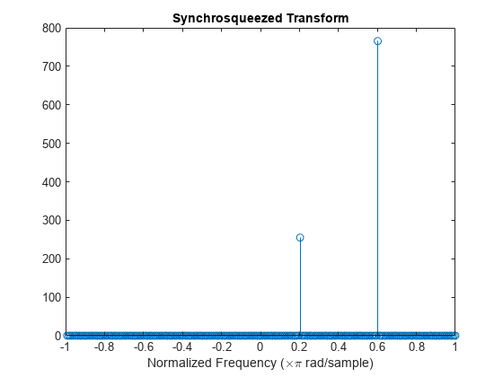
The Fourier synchrosqueezed transform concentrates the energy content of the signal at the estimated instantaneous frequencies.

stem(sw/pi,abs(ss(:,128)))
xlabel("Normalized Frequency (\times\pi rad/sample)")
title("Synchrosqueezed Transform")

Figure contains an axes object. The axes object with title Synchrosqueezed Transform, xlabel Normalized Frequency ( times pi blank rad/sample) contains an object of type stem.

The synchrosqueezed estimates of instantaneous frequency are valid only if the sinusoids are separated by more than 2Δ, where

Δ=1σ2log2

for a Gaussian window and σ is the standard deviation.

Repeat the previous calculation, but now specify that the second sinusoid has a normalized frequency of ω0+1.9Δ rad/sample.

D = sqrt(2*log(2))/rstdev;

w1 = w0+1.9*D;

x = exp(1j*w0*n)+3*exp(1j*w1*n);

[s,w,t] = spectrogram(x,gausswin(Nw,alpha),Nw-1,nfft,"centered");
instransf = abs(s(:,20));

plot(w/pi,instransf)
hold on
plot(w/pi,[1 3]*amp.*exp(-rstdev^2/2*(w-[w0 w1]).^2),"--")
hold off
xlabel("Normalized Frequency (\times\pi rad/sample)")
legend(["Transform" "First sinusoid" "Second sinusoid"],Location="best")

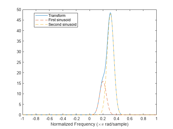
Figure contains an axes object. The axes object with xlabel Normalized Frequency ( times pi blank rad/sample) contains 3 objects of type line. These objects represent Transform, First sinusoid, Second sinusoid.

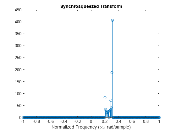
The Fourier synchrosqueezed transform cannot resolve the sinusoids well because |ω1-ω0|<2Δ. The spectral estimates decrease significantly in value.

[ss,sw,st] = fsst(x,[],gausswin(Nw,alpha));

stem(sw/pi,abs(ss(:,128)))
xlabel("Normalized Frequency (\times\pi rad/sample)")
title("Synchrosqueezed Transform")

Figure contains an axes object. The axes object with title Synchrosqueezed Transform, xlabel Normalized Frequency ( times pi blank rad/sample) contains an object of type stem.

Load a speech signal sampled at Fs=7418Hz. The file contains a recording of a female voice saying the word "MATLAB®."

load mtlb

% To hear, type sound(mtlb,Fs)

Compute the synchrosqueezed transform of the signal. Use a Hann window of length 256. Display the time on the x-axis and the frequency on the y-axis.

fsst(mtlb,Fs,hann(256),'yaxis')

Figure contains an axes object. The axes object with title Fourier Synchrosqueezed Transform, xlabel Time (ms), ylabel Frequency (kHz) contains an object of type image.

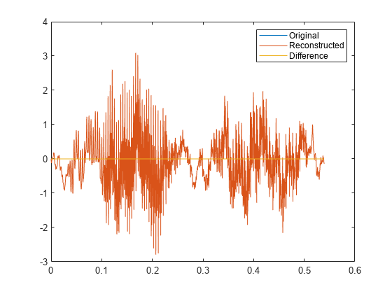
Use ifsst to invert the transform. Compare the original and reconstructed signals.

sst = fsst(mtlb,Fs,hann(256));

xrc = ifsst(sst,hann(256));

plot((0:length(mtlb)-1)/Fs,[mtlb xrc xrc-mtlb])
legend('Original','Reconstructed','Difference')

Figure contains an axes object. The axes object contains 3 objects of type line. These objects represent Original, Reconstructed, Difference.

% To hear, type sound(xrc-mtlb,Fs)

Input Arguments

collapse all

Input signal, specified as a vector.

Example: cos(pi/4*(0:159))+randn(1,160) specifies a sinusoid embedded in white Gaussian noise.

Data Types: single | double
Complex Number Support: Yes

Sample rate, specified as a positive scalar. The sample rate is the number of samples per unit time. If the unit of time is seconds, then the sample rate is in Hz.

Data Types: double | single

Sample time, specified as a duration scalar. The sample time is the time elapsed between consecutive samples of x.

Data Types: duration

Window used to divide the signal into segments, specified as an integer or as a row or column vector.

  • If window is an integer, then fsst divides x into segments of length window and windows each segment with a Kaiser window of that length and β = 10. The overlap between adjacent segments is window – 1.

  • If window is a vector, then fsst divides x into segments of the same length as the vector and windows each segment using window. The overlap between adjacent segments is length(window) – 1.

  • If window is not specified, then fsst divides x into segments of length 256 and windows each segment with a 256-sample Kaiser window with β = 10. The overlap between adjacent segments is 255. If x has fewer than 256 samples, then the function uses a single Kaiser window with the same length as x and β = 10.

For a list of available windows, see Windows.

Example: hann(N+1) and (1-cos(2*pi*(0:N)'/N))/2 both specify a Hann window of length N + 1.

Data Types: double | single

Frequency display axis, specified as 'xaxis' or 'yaxis'.

  • 'xaxis' — Displays frequency on the x-axis and time on the y-axis.

  • 'yaxis' — Displays frequency on the y-axis and time on the x-axis.

This argument is ignored if you call fsst with output arguments.

Output Arguments

collapse all

Fourier synchrosqueezed transform, returned as a matrix. The number of columns of s equals the length of x. Time increases across the columns of s and frequency increases down the rows of s, starting from zero. If x is real, then its synchrosqueezed spectrum is one-sided. If x is complex, then its synchrosqueezed spectrum is two-sided and centered.

Normalized frequencies, returned as a vector. The length of w equals the number of rows in s.

Sample numbers, returned as a vector. The length of n equals the number of columns in s. Each sample number in n is the midpoint of a windowed segment of x.

Cyclical frequencies, returned as a vector. The length of f equals the number of rows in  s.

Time instants, returned as a vector. The length of t equals the number of columns in s. Each time value in t is the midpoint of a windowed segment of x.

More About

collapse all

Fourier Synchrosqueezed Transform

Many real-world signals such as speech waveforms, machine vibrations, and physiologic signals can be expressed as a superposition of amplitude-modulated and frequency-modulated modes. For time-frequency analysis, it is convenient to express such signals as sums of analytic signals through

f(t)=k=1Kfk(t)=k=1KAk(t)ej2πϕk(t).

The phases ϕk(t) have time derivatives k(t)/dt that correspond to instantaneous frequencies. When the exact phases are unknown, you can use the Fourier synchrosqueezed transform to estimate them.

The Fourier synchrosqueezed transform is based on the short-time Fourier transform implemented in the spectrogram function. For certain kinds of nonstationary signals, the synchrosqueezed transform resembles the reassigned spectrogram because it generates sharper time-frequency estimates than the conventional transform. The fsst function determines the short-time Fourier transform of a function, f, using a spectral window, g, and computing

Vgf(t,η)=f(x)g(xt)ej2πη(xt)dx.

Unlike the conventional definition, this definition has an extra factor of ej2πηt. The transform values are then “squeezed” so that they concentrate around curves of instantaneous frequency in the time-frequency plane. The resulting synchrosqueezed transform is of the form

Tgf(t,ω)=Vgf(t,η)δ(ωΩgf(t,η))dη,

where the instantaneous frequencies are estimated with the “phase transform”

Ωgf(t,η)=1j2πtVgf(t,η)Vgf(t,η)=η1j2πVg/tf(t,η)Vgf(t,η).

The transform in the denominator decreases the influence of the window. To see a simple example, refer to Detect Closely Spaced Sinusoids with the Fourier Synchrosqueezed Transform. The definition of Tgf(t,ω) differs by a factor of 1/g(0) from other expressions found in the literature. fsst incorporates the factor in the mode-reconstruction step.

Unlike the reassigned spectrogram, the synchrosqueezed transform is invertible and thus can reconstruct the individual modes that compose the signal. Invertibility imposes some constraints on the computation of the short-time Fourier transform:

  • The number of DFT points is equal to the length of the specified window.

  • The overlap between adjoining windowed segments is one less than the window length.

  • The reassignment is performed only in frequency.

To find the modes, integrate the synchrosqueezed transform over a small frequency interval around Ωgf(t,η):

fk(t)1g(0)|ωΩk(t)|<εTgf(t,ω)dω,

where ɛ is a small number.

The synchrosqueezed transform produces narrow ridges compared to the windowed short-time Fourier transform. However, the width of the short-time transform still affects the ability of the synchrosqueezed transform to separate modes. To be resolvable, the modes must obey these conditions:

  1. For each mode, the frequency must be strictly greater than the rate of change of the amplitude: dϕk(t)dt>dAk(t)dt for all k.

  2. Distinct modes must be separated by at least the frequency bandwidth of the window. If the support of the window is the interval [–Δ,Δ], then |dϕk(t)dtdϕm(t)dt|>2Δ for km.

For an illustration, refer to Detect Closely Spaced Sinusoids with the Fourier Synchrosqueezed Transform.
References

[1] Auger, François, Patrick Flandrin, Yu-Ting Lin, Stephen McLaughlin, Sylvain Meignen, Thomas Oberlin, and Hau-Tieng Wu. "Time-Frequency Reassignment and Synchrosqueezing: An Overview." IEEE® Signal Processing Magazine. Vol. 30, November 2013, pp. 32–41.

[2] Oberlin, Thomas, Sylvain Meignen, and Valérie Perrier. "The Fourier-based Synchrosqueezing Transform." Proceedings of the 2014 IEEE International Conference on Acoustics, Speech, and Signal Processing (ICASSP), pp. 315–319.

[3] Thakur, Gaurav, and Hau-Tieng Wu. "Synchrosqueezing-based Recovery of Instantaneous Frequency from Nonuniform Samples." SIAM Journal of Mathematical Analysis. Vol. 43, 2011, pp. 2078–2095.

Extended Capabilities

Version History

Introduced in R2016b