Trajectory Control Modeling with Inverse Kinematics
This Simulink example demonstrates how the Inverse Kinematics block can drive a manipulator along a specified trajectory. The desired trajectory is specified as a series of tightly-spaced poses for the end effector of the manipulator. Trajectory generation and waypoint definition represents many robotics applications like pick and place operation, calculating trajectories from spatial acceleration and velocity profiles, or even mimicking external observations of key frames using cameras and computer vision. Once a trajectory is generated, the Inverse Kinematics block is used to translate this to a joint-space trajectory, which can then be used to simulate the dynamics of the manipulator and controller.
Model Overview
Load the model to see how it is constructed.
open_system('IKTrajectoryControlExample.slx');The model is composed of four primary operations:
Target Pose Generation
Inverse Kinematics
Manipulator Dynamics
Pose Measurement
Target Pose Generation
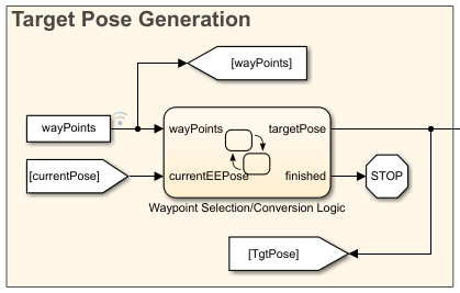
This Stateflow chart selects which waypoint is the current objective for the manipulator. The chart adjusts the target to the next waypoint once the manipulator gets to within a tolerance of the current objective. The chart also converts and assembles the components of the waypoint into a homogenous transformation through the eul2tform function. Once there are no more waypoints to select, the chart terminates the simulation.
Inverse Kinematics
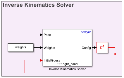
Inverse kinematics calculated a set of joint angles to produce a desired pose for an end effector. Use the Inverse Kinematicswith a rigidBodyTree model and specify the target pose of the end effect as a homogenous transformation. Specify a series of weights for the relative tolerance constraints on the position and orientation of the solution, and give an initial estimate of the joint positions. The block outputs a vector of joint positions that produce the desired pose from the rigidBodyTree model specified in the block parameters. To ensure smooth continuity of the solutions, the previous configuration solution is used as the starting position for the solver. This also reduces the redundancy of calculations if the target pose has not updated since the last simulation time step.
Manipulator Dynamics
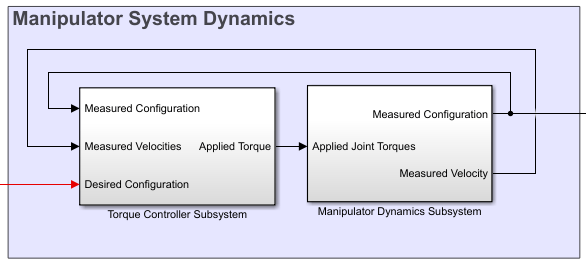
The manipulator dynamics consists of two components, a controller to generate torque signals and a dynamics model to model the dynamics of the manipulator given these torque signals. The controller in the example uses a feed-forward component calculated through the inverse dynamics of the manipulator and a feedback PD controller to correct for error. The model of the manipulator uses the Forward Dynamics block that works with a rigidBodyTree object. For more sophisticated dynamics and visualization techniques, consider utilizing tools from the Control Systems Toolbox™ blockset and Simscape Multibody™ to replace the Forward Dynamics block.
Pose Measurement
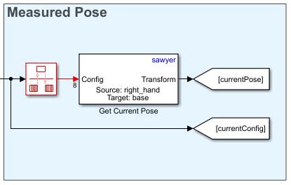
The pose measurement takes the joint angle readings from the manipulator model and converts them into a homogenous transform matrix to be used as feedback in the Waypoint Selection section.
Manipulator Definition
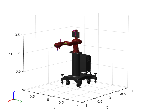
The manipulator used for this example is the Rethink Sawyer™ robot manipulator. The rigidBodyTree object that describes the manipulator is imported from a URDF (unified robot description format) file using importrobot.
% Import the manipulator as a rigidBodyTree Object
sawyer = importrobot('sawyer.urdf');
sawyer.DataFormat = 'column';

% Define end-effector body name
eeName = 'right_hand';

% Define the number of joints in the manipulator
numJoints = 8;

% Visualize the manipulator
show(sawyer);
xlim([-1.00 1.00])
ylim([-1.00 1.00]);
zlim([-1.02 0.98]);
view([128.88 10.45]);
Waypoint Generation
In this example, the goal of the manipulator is to be able to trace out the boundaries of the coins detected in the image, coins.png. First, the image is processed to find the boundaries of the coins.
I = imread('coins.png');
bwBoundaries = imread('coinBoundaries.png');

figure
subplot(1,2,1)
imshow(I,'Border','tight')
title('Original Image')

subplot(1,2,2)
imshow(bwBoundaries,'Border','tight')
title('Processed Image with Boundary Detection')
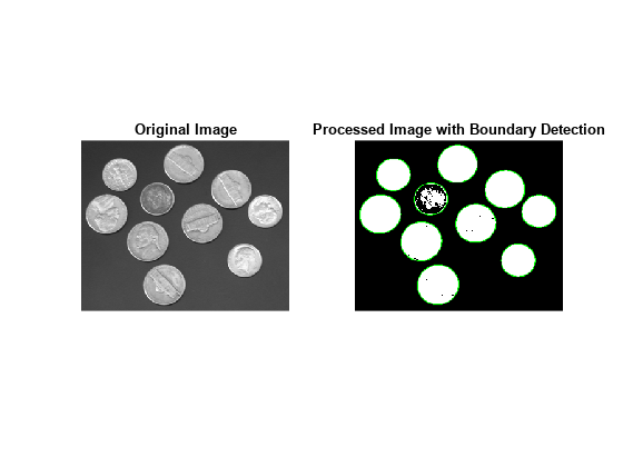
After the image processing, the edges of the coins are extracted as pixel locations. The data is loaded in from the MAT-file, boundaryData. boundaries is a cell array where each cell contains an array describing the pixel coordinates for a single detected boundary. A more comprehensive view of how to generate this data can be found in the example, "Boundary Tracing in Images" (requires Image Processing Toolbox).
load boundaryData.mat boundaries
whos boundaries
  Name             Size            Bytes  Class    Attributes

  boundaries      10x1             25376  cell
To map this data to the world frame, we need to define where the image is located and the scaling between pixel coordinates and spatial coordinates.
% Image origin coordinates
imageOrigin = [0.4,0.2,0.08];

% Scale factor to convert from pixels to physical distance
scale = 0.0015;
The Euler angles for the desired end effector orientation at each point must also be defined.
eeOrientation = [0, pi, 0];
In this example the orientation is chosen such that the end effector is always perpendicular to the plane of the image.
Once this information is defined each set of desired coordinates and Euler angles can be compiled into a waypoint. Each waypoint is represented as a six-element vector whose first three elements correspond to the desired xyz-positions of the manipulator in the world frame. The last three elements correspond to the ZYX Euler angles of the desired orientation.
The waypoints are concatenated to form an n-by-6 array, where n is the total number of poses in the trajectory. Each row in the array corresponds to a waypoint in the trajectory.
% Clear previous waypoints and begin building wayPoint array
clear wayPoints

% Start just above image origin
waypt0 = [imageOrigin + [0 0 .2],eeOrientation];

% Touch the origin of the image
waypt1 = [imageOrigin,eeOrientation];

% Interpolate each element for smooth motion to the origin of the image
for i = 1:6

    interp = linspace(waypt0(i),waypt1(i),100);
    wayPoints(:,i) = interp';

end
In total, there are 10 coins. For simplicity and speed, a smaller subset of coins can be traced by limiting the total number passed to the waypoints. The number of coins this code traces in the images is three.
% Define the number of coins to trace
numTraces = 3;

% Assemble the waypoints for boundary tracing
for i = 1:min(numTraces, size(boundaries,1))

    %Select a boundary and map to physical size
    segment = boundaries{i}*scale;

    % Pad data for approach waypoint and lift waypoint between boundaries
    segment = [segment(1,:); segment(:,:); segment(end,:)];

    % Z-offset for moving between boundaries
    segment(1,3) = .02;
    segment(end,3) = .02;

    % Translate to origin of image
    cartesianCoord = imageOrigin + segment;

    % Repeat desired orientation to match the number of waypoints being added
    eulerAngles = repmat(eeOrientation,size(segment,1),1);

    % Append data to end of previous wayPoints
    wayPoints = [wayPoints;
                 cartesianCoord, eulerAngles];
end
This array is the primary input to the model.
Model Setup
Several parameters must be initialized before the model can be run.
% Initialize size of q0, the robot joint configuration at t=0. This will
% later be replaced by the first waypoint.
q0 = zeros(numJoints,1);

% Define a sampling rate for the simulation.
Ts = .01;

% Define a [1x6] vector of relative weights on the orientation and
% position error for the inverse kinematics solver.
weights = ones(1,6);

% Transform the first waypoint to a Homogenous Transform Matrix for initialization
initTargetPose = eul2tform(wayPoints(1,4:6));
initTargetPose(1:3,end) = wayPoints(1,1:3)';

% Solve for q0 such that the manipulator begins at the first waypoint
ik = inverseKinematics('RigidBodyTree',sawyer);
[q0,solInfo] = ik(eeName,initTargetPose,weights,q0);
Simulate the Manipulator Motion
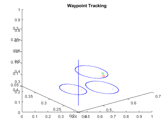
To simulate the model, use the sim command. The model generates the output dataset, jointData and shows the progress in two plots:
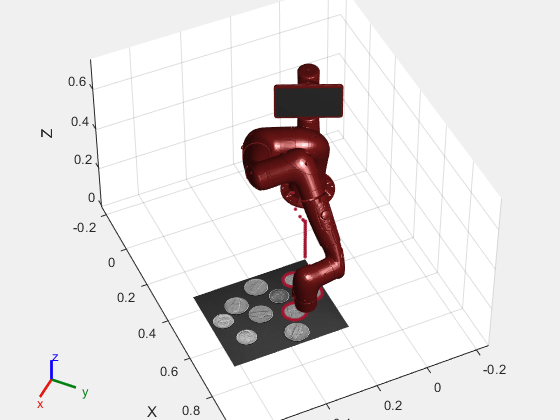
The X Y Plot shows a top-down view of the tracing motions of the manipulator. The lines between the circles occur as the manipulator transitions from one coin outline to the next.
The Waypoint Tracking plot visualizes the progress in 3D. The green dot indicates the target position. The red dot indicates the actual end-effector position achieved by the end effector using feedback control.
% Close currently open figures
close all

% Open & simulate the model
open_system('IKTrajectoryControlExample.slx');
sim('IKTrajectoryControlExample.slx');
Visualize the Results
The model outputs two datasets that can be used for visualization after simulation. The joint configurations are provided as jointData. The robot end-effector poses are output as poseData.
% Remove unnecessary meshes for faster visualization
clearMeshes(sawyer);

% Data for mapping image
[m,n] = size(I);

[X,Y] = meshgrid(0:m,0:n);
X = imageOrigin(1) + X*scale;
Y = imageOrigin(2) + Y*scale;

Z = zeros(size(X));
Z = Z + imageOrigin(3);

% Close all open figures
close all

% Initialize a new figure window
figure;
set(gcf,'Visible','on');

% Plot the initial robot position
show(sawyer, jointData(1,:)');
hold on

% Initialize end effector plot position
p = plot3(0,0,0,'.');
warp(X,Y,Z,I');

% Change view angle and axis
view(65,45)
axis([-.25 1 -.25 .75 0 0.75])

% Iterate through the outputs at 10-sample intervals to visualize the results
for j = 1:10:length(jointData)
    % Display manipulator model
    show(sawyer,jointData(j,:)', 'Frames', 'off', 'PreservePlot', false);

    % Get end effector position from homoegenous transform output
    pos = poseData(1:3,4,j);

    % Update end effector position for plot
    p.XData = [p.XData pos(1)];
    p.YData = [p.YData pos(2)];
    p.ZData = [p.ZData pos(3)];

    % Update figure
    drawnow
end
