Train DDPG Agent for Adaptive Cruise Control
This example shows how to train a deep deterministic policy gradient (DDPG) agent for adaptive cruise control (ACC) in Simulink®. For more information on DDPG agents, see Deep Deterministic Policy Gradient (DDPG) Agents.
Simulink Model
The reinforcement learning environment for this example is the simple longitudinal dynamics for an ego car and lead car. The training goal is to make the ego car travel at a set velocity while maintaining a safe distance from lead car by controlling longitudinal acceleration and braking. This example uses the same vehicle model as the Adaptive Cruise Control System Using Model Predictive Control (Model Predictive Control Toolbox) example.
Specify the initial position and velocity for the two vehicles.
x0_lead = 50;   % initial position for lead car (m)
v0_lead = 25;   % initial velocity for lead car (m/s)
x0_ego = 10;    % initial position for ego car (m)
v0_ego = 20;    % initial velocity for ego car (m/s)
Specify standstill default spacing (m), time gap (s) and driver-set velocity (m/s).
D_default = 10;
t_gap = 1.4;
v_set = 30;
To simulate the physical limitations of the vehicle dynamics, constraint the acceleration to the range [–3,2] m/s^2.
amin_ego = -3;
amax_ego = 2;
Define the sample time Ts and simulation duration Tf in seconds.
Ts = 0.1;
Tf = 60;
Open the model.
mdl = "rlACCMdl";
open_system(mdl)
agentblk = mdl + "/RL Agent";

For this model:
The acceleration action signal from the agent to the environment is from –3 to 2 m/s^2.
The reference velocity for the ego car is defined as follows. If the relative distance is less than the safe distance, the ego car tracks the minimum of the lead car velocity and driver-set velocity. In this manner, the ego car maintains some distance from the lead car. If the relative distance is greater than the safe distance, the ego car tracks the driver-set velocity. In this example, the safe distance is defined as a linear function of the ego car longitudinal velocity ; that is, . The safe distance determines the reference tracking velocity for the ego car.
The observations from the environment are the velocity error , its integral , and the ego car longitudinal velocity .
The simulation is terminated when longitudinal velocity of the ego car is less than 0, or the relative distance between the lead car and ego car becomes less than 0.
The reward , provided at every time step , is
where is the control input from the previous time step. The logical value if velocity error ; otherwise, .
Create Environment Interface
Create a reinforcement learning environment interface for the model.
Create the observation specification.
obsInfo = rlNumericSpec([3 1], ...
    LowerLimit=-inf*ones(3,1), ...
    UpperLimit=inf*ones(3,1));
obsInfo.Name = "observations";
obsInfo.Description = ...
    "velocity error and ego velocity";
Create the action specification.
actInfo = rlNumericSpec([1 1], ...
    LowerLimit=-3,UpperLimit=2);
actInfo.Name = "acceleration";
Create the environment interface.
env = rlSimulinkEnv(mdl,agentblk,obsInfo,actInfo);
To define the initial condition for the position of the lead car, specify an environment reset function using an anonymous function handle. The reset function localResetFcn, which is defined at the end of the example, randomizes the initial position of the lead car.
env.ResetFcn = @(in)localResetFcn(in);
Fix the random generator seed for reproducibility.
rng("default")Create DDPG agent
DDPG agents use a parametrized Q-value function critic to estimate the value of the policy. A Q-value function takes the current observation and an action as inputs and returns a single scalar as output (the estimated discounted cumulative long-term reward given the action from the state corresponding to the current observation, and following the policy thereafter).
To model the parametrized Q-value function within the critic, use a neural network with two input layers (one for the observation channel, as specified by obsInfo, and the other for the action channel, as specified by actInfo) and one output layer (which returns the scalar value).
Define each network path as an array of layer objects. Use prod(obsInfo.Dimension) and prod(actInfo.Dimension) to return the number of dimensions of the observation and action spaces.
Assign names to the input and output layers of each path. These names allow you to connect the paths and then later explicitly associate the network input and output layers with the appropriate environment channel.
L = 48; % number of neurons

% Main path
mainPath = [
    featureInputLayer( ...
        prod(obsInfo.Dimension), ...
        Name="obsInLyr")
    fullyConnectedLayer(L)
    reluLayer
    fullyConnectedLayer(L)
    additionLayer(2,Name="add")
    reluLayer
    fullyConnectedLayer(L)
    reluLayer
    fullyConnectedLayer(1,Name="QValLyr")
    ];

% Action path
actionPath = [
    featureInputLayer( ...
        prod(actInfo.Dimension), ...
        Name="actInLyr")
    fullyConnectedLayer(L,Name="actOutLyr")
    ];

% Assemble layers into a layergraph object
criticNet = layerGraph(mainPath);
criticNet = addLayers(criticNet, actionPath);

% Connect layers
criticNet = connectLayers(criticNet,"actOutLyr","add/in2");

% Convert to dlnetwork and display number of weights
criticNet = dlnetwork(criticNet);
summary(criticNet)
   Initialized: true

   Number of learnables: 5k

   Inputs:
      1   'obsInLyr'   3 features
      2   'actInLyr'   1 features
View the critic network configuration.
plot(criticNet)

Create the critic approximator object using criticNet, the environment observation and action specifications, and the names of the network input layers to be connected with the environment observation and action channels. For more information, see rlQValueFunction.
critic = rlQValueFunction(criticNet,obsInfo,actInfo,...
    ObservationInputNames="obsInLyr",ActionInputNames="actInLyr");
DDPG agents use a parametrized deterministic policy over continuous action spaces, which is learned by a continuous deterministic actor. This actor takes the current observation as input and returns as output an action that is a deterministic function of the observation.
To model the parametrized policy within the actor, use a neural network with one input layer (which receives the content of the environment observation channel, as specified by obsInfo) and one output layer (which returns the action to the environment action channel, as specified by actInfo).
Define the network as an array of layer objects. Use a tanhLayer followed by a scalingLayer to scale the network output to the action range.
actorNet = [
    featureInputLayer(prod(obsInfo.Dimension))
    fullyConnectedLayer(L)
    reluLayer
    fullyConnectedLayer(L)
    reluLayer
    fullyConnectedLayer(L)
    reluLayer
    fullyConnectedLayer(prod(actInfo.Dimension))
    tanhLayer
    scalingLayer(Scale=2.5,Bias=-0.5)
    ];
Convert to dlnetwork and display the number of weights.
actorNet = dlnetwork(actorNet);
summary(actorNet)
   Initialized: true

   Number of learnables: 4.9k

   Inputs:
      1   'input'   3 features
Create the actor using actorNet and the observation and action specifications. For more information on continuous deterministic actors, see rlContinuousDeterministicActor.
actor = rlContinuousDeterministicActor(actorNet, ...
    obsInfo,actInfo);
Specify training options for the critic and the actor using rlOptimizerOptions.
criticOptions = rlOptimizerOptions( ...
    LearnRate=1e-3, ...
    GradientThreshold=1, ...
    L2RegularizationFactor=1e-4);
actorOptions = rlOptimizerOptions( ...
    LearnRate=1e-4, ...
    GradientThreshold=1, ...
    L2RegularizationFactor=1e-4);
Specify the DDPG agent options using rlDDPGAgentOptions, include the training options for the actor and critic.
agentOptions = rlDDPGAgentOptions(...
    SampleTime=Ts,...
    ActorOptimizerOptions=actorOptions,...
    CriticOptimizerOptions=criticOptions,...
    ExperienceBufferLength=1e6);
You can also set or modify the agent options using dot notation.
agentOptions.NoiseOptions.Variance = 0.6;
agentOptions.NoiseOptions.VarianceDecayRate = 1e-5;
Alternatively, you can create the agent first, and then access its option object and modify the options using dot notation.
Create the DDPG agent using the specified actor representation, critic representation, and agent options. For more information, see rlDDPGAgent.
agent = rlDDPGAgent(actor,critic,agentOptions);
Train Agent
To train the agent, first specify the training options. For this example, use the following options:
Run each training episode for at most
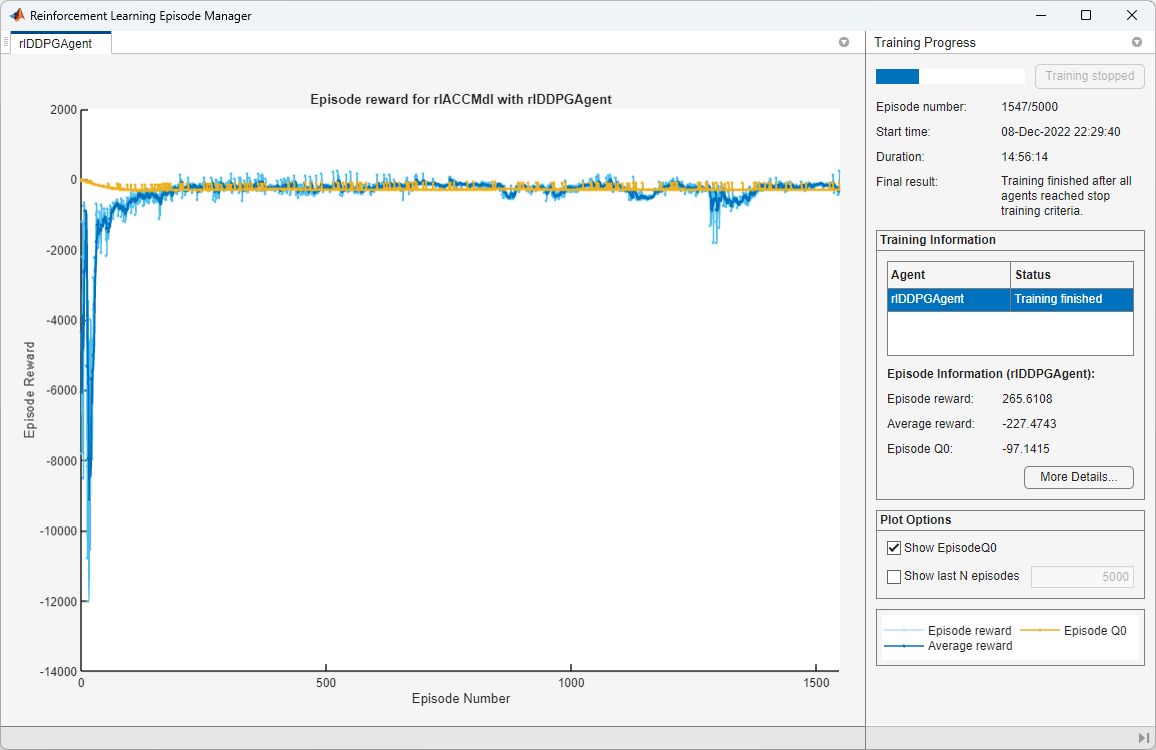
5000episodes, with each episode lasting at most 600 time steps.Display the training progress in the Episode Manager dialog box.
Stop training when the agent receives an episode reward greater than 260.
For more information, see rlTrainingOptions.
maxepisodes = 5000;
maxsteps = ceil(Tf/Ts);
trainingOpts = rlTrainingOptions(...
    MaxEpisodes=maxepisodes,...
    MaxStepsPerEpisode=maxsteps,...
    Verbose=false,...
    Plots="training-progress",...
    StopTrainingCriteria="EpisodeReward",...
    StopTrainingValue=260);
Train the agent using the train function. Training is a computationally intensive process that takes several minutes to complete. To save time while running this example, load a pretrained agent by setting doTraining to false. To train the agent yourself, set doTraining to true.
doTraining = false;

if doTraining
    % Train the agent.
    trainingStats = train(agent,env,trainingOpts);
else
    % Load a pretrained agent for the example.
    load("SimulinkACCDDPG.mat","agent")
end

Simulate DDPG Agent
To validate the performance of the trained agent, you can simulate the agent within the Simulink environment using the following commands. For more information on agent simulation, see rlSimulationOptions and sim.
simOptions = rlSimulationOptions(MaxSteps=maxsteps);
experience = sim(env,agent,simOptions);
To demonstrate the trained agent using deterministic initial conditions, simulate the model in Simulink.
x0_lead = 80;
sim(mdl)
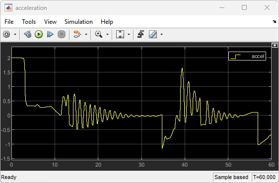
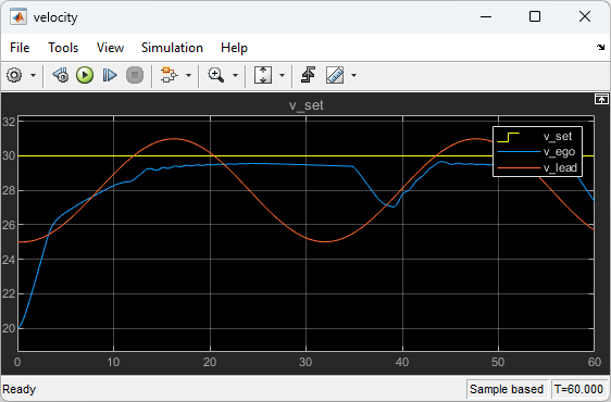
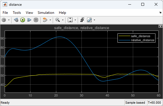
The following plots show the simulation results when lead car is 70 (m) ahead of the ego car.
In the first 35 seconds, the relative distance is greater than the safe distance (bottom plot), so the ego car tracks set velocity (middle plot). To speed up and reach the set velocity, acceleration is initially positive (top plot).
From 35 to 48 seconds, the relative distance is less than the safe distance (bottom plot), so the ego car tracks the minimum of the lead velocity and set velocity. To slow down and track the lead car velocity, the acceleration turns negative from 35 to approximately 37 seconds (top plot). Afterwards, the ego car adjusts its acceleration to keep on tracking either the minimum between the lead velocity and the set velocity, or the set velocity, depending on whether the relative distance is deemed to be safe or not.


Close the Simulink model.
bdclose(mdl)
Reset Function
function in = localResetFcn(in)
% Reset the initial position of the lead car.
in = setVariable(in,"x0_lead",40+randi(60,1,1));
end
See Also
Functions
train|sim|rlSimulinkEnv
Objects
rlDDPGAgent|rlDDPGAgentOptions|rlQValueFunction|rlContinuousDeterministicActor|rlTrainingOptions|rlSimulationOptions|rlOptimizerOptions
Blocks
Related Examples
- Train Multiple Agents for Path Following Control
- Train DDPG Agent for Path-Following Control
- Train DQN Agent for Lane Keeping Assist
- Adaptive Cruise Control System Using Model Predictive Control (Model Predictive Control Toolbox)
