bat365 Homepage

Nonlinear Heat Transfer in Thin Plate

This example shows how to perform a heat transfer analysis of a thin plate.

The plate is square, and the temperature is fixed along the bottom edge. The other three edges are insulated, there is no heat transfer from these edges. Heat is transferred from both the top and bottom faces of the plate by convection and radiation. Because radiation is included, the problem is nonlinear. One of the purposes of this example is to show how to handle nonlinearities in PDE problems.

These example shows how to perform both a steady state and a transient analysis. In a steady state analysis, the example computes the final temperature at different points in the plate after it has reached an equilibrium state. In a transient analysis, the example computes the temperature in the plate as a function of time. The transient analysis section of the example also finds how long it takes for the plate to reach an equilibrium temperature.

Heat Transfer Equations for the Plate

The plate has planar dimensions one meter by one meter and is 1 cm thick. Because the plate is relatively thin compared with the planar dimensions, the temperature can be assumed constant in the thickness direction; the resulting problem is 2D.

Convection and radiation heat transfer are assumed to take place between the two faces of the plate and a specified ambient temperature.

The amount of heat transferred from each face per unit area due to convection is defined as

$Q_{c} = h_{c} (T - T_{a})$

where $T_{a}$ is the ambient temperature, $T$ is the temperature at a particular x and y location on the plate surface, and $h_{c}$ is a specified convection coefficient.

The amount of heat transferred from each face per unit area due to radiation is defined as

$Q_{r} = ϵ σ (T^{4} - T_{a}^{4})$

where $ϵ$ is the emissivity of the face and $σ$ is the Stefan-Boltzmann constant. Because the heat transferred due to radiation is proportional to the fourth power of the surface temperature, the problem is nonlinear.

The PDE describing the temperature in this thin plate is

$ρ C_{p} t_{z} \frac{\partial T}{\partial t} - k t_{z} \nabla^{2} T + 2 Q_{c} + 2 Q_{r} = 0$

where $ρ$ is the material density, $C_{p}$ is the specific heat, $t_{z}$ is the plate thickness, and the factors of two account for the heat transfer from both plate faces.

Rewrite this equation in the form required by the toolbox:

$ρ C_{p} t_{z} \frac{\partial T}{\partial t} - k t_{z} \nabla^{2} T + 2 h_{c} T + 2 ϵ σ T^{4} = 2 h_{c} T_{a} + 2 ϵ σ T_{a}^{4}$

Problem Setup

Specify these properties for a copper plate.

k = 400; % thermal conductivity of copper, W/(m-K)
rho = 8960; % density of copper, kg/m^3
specificHeat = 386; % specific heat of copper, J/(kg-K)
thick = .01; % plate thickness in meters
stefanBoltz = 5.670373e-8; % Stefan-Boltzmann constant, W/(m^2-K^4)
hCoeff = 1; % Convection coefficient, W/(m^2-K)
% The ambient temperature is assumed to be 300 degrees-Kelvin.
ta = 300;
emiss = .5; % emissivity of the plate surface

Create a model.

model = createpde;

Define a unit square geometry.

width = 1; 
height = 1;
gdm = [3 4 0 width width 0 0 0 height height]';
g = decsg(gdm,'S1',('S1')');

Include the geometry in the model.

geometryFromEdges(model,g);

Plot the geometry and display the edge labels.

figure; 
pdegplot(model,"EdgeLabels","on"); 
axis([-.1 1.1 -.1 1.1]);
title("Geometry With Edge Labels Displayed")

Figure contains an axes object. The axes object with title Geometry With Edge Labels Displayed contains 5 objects of type line, text.

Specify the coefficients.

c = thick*k;
f = 2*hCoeff*ta + 2*emiss*stefanBoltz*ta^4;
d = thick*rho*specificHeat;

Because of the radiation boundary condition, the coefficient a is a function of the temperature u.

a = @(~,state) 2*hCoeff + 2*emiss*stefanBoltz*state.u.^3;
specifyCoefficients(model,"m",0,"d",0,"c",c,"a",a,"f",f);

Apply the boundary conditions. For the insulated edges, keep the default zero Neumann boundary condition. For the bottom edge (edge 1), use the Dirichlet boundary condition to set the temperature to 1000 K.

applyBoundaryCondition(model,"dirichlet","Edge",1,"u",1000);

Generate and plot a mesh.

hmax = .1; % element size
msh = generateMesh(model,"Hmax",hmax);
figure; 
pdeplot(model); 
axis equal
xlabel("X-coordinate, meters")
ylabel("Y-coordinate, meters")

Figure contains an axes object. The axes object with xlabel X-coordinate, meters, ylabel Y-coordinate, meters contains 2 objects of type line.

Steady State Solution

Solve the problem by using solvepde.

R = solvepde(model);
u = R.NodalSolution;
figure; 
pdeplot(model,"XYData",u,"Contour","on","ColorMap","jet");
title("Temperature In The Plate, Steady State Solution")
xlabel("X-coordinate, meters")
ylabel("Y-coordinate, meters")
axis equal

Figure contains an axes object. The axes object with title Temperature In The Plate, Steady State Solution, xlabel X-coordinate, meters, ylabel Y-coordinate, meters contains 12 objects of type patch, line.

p = msh.Nodes;
plotAlongY(p,u,0);
title("Temperature As a Function of the Y-Coordinate")
xlabel("Y-coordinate, meters")
ylabel("Temperature, degrees-Kelvin")

Figure contains an axes object. The axes object with title Temperature As a Function of the Y-Coordinate, xlabel Y-coordinate, meters, ylabel Temperature, degrees-Kelvin contains an object of type line.

fprintf(['Temperature at the top edge of the plate =' ...
         ' %5.1f degrees-K\n'],u(4));

Temperature at the top edge of the plate = 449.8 degrees-K

Transient Solution

Include the d coefficient.

specifyCoefficients(model,"m",0,"d",d,"c",c,"a",a,"f",f);
endTime = 5000;
tlist = 0:50:endTime;

Set the initial temperature on the entire plate to 300 K.

setInitialConditions(model,300);

Set the initial temperature on the bottom edge to the value of the constant boundary condition, 1000 K.

setInitialConditions(model,1000,"Edge",1);

Set the following solver options.

model.SolverOptions.RelativeTolerance = 1.0e-3; 
model.SolverOptions.AbsoluteTolerance = 1.0e-4;

Solve the problem by using solvepde.

R = solvepde(model,tlist);
u = R.NodalSolution;
figure; 
plot(tlist,u(3,:)); 
grid on
title(["Temperature Along the Top Edge of " ...
       "the Plate as a Function of Time"])
xlabel("Time, seconds")
ylabel("Temperature, degrees-Kelvin")

Figure contains an axes object. The axes object with title Temperature Along the Top Edge of the Plate as a Function of Time, xlabel Time, seconds, ylabel Temperature, degrees-Kelvin contains an object of type line.

figure;
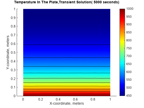
pdeplot(model,"XYData",u(:,end),"Contour","on","ColorMap","jet");
title(sprintf(['Temperature In The Plate,' ...
               'Transient Solution( %d seconds)\n'],tlist(1,end)));
xlabel("X-coordinate, meters")
ylabel("Y-coordinate, meters")
axis equal;

Figure contains an axes object. The axes object with xlabel X-coordinate, meters, ylabel Y-coordinate, meters contains 12 objects of type patch, line.

fprintf(['\nTemperature at the top edge(t = %5.1f secs) = ' ...
         '%5.1f degrees-K\n'],tlist(1,end),u(4,end));

Temperature at the top edge(t = 5000.0 secs) = 448.1 degrees-K

Summary

The plots of temperature in the plate from the steady state and transient solution at the ending time are very close. That is, after around 5000 seconds, the transient solution has reached the steady state values. The temperatures from the two solutions at the top edge of the plate agree to within one percent.