Steady-State Solution

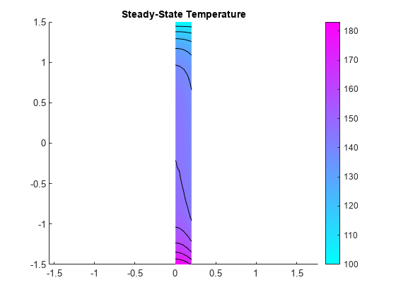
First, compute the steady-state solution. If the final time in the transient analysis is sufficiently large, the transient solution at the final time must be close to the steady state solution. By comparing these two results, you can check the accuracy of the transient analysis.

Create a steady-state thermal model for solving an axisymmetric problem.

thermalmodel = createpde("thermal","steadystate-axisymmetric");

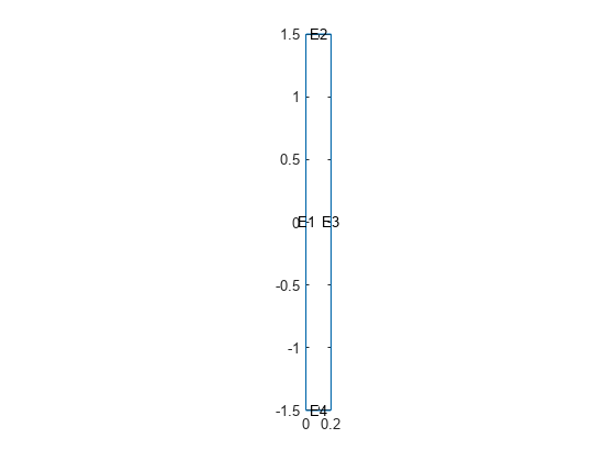
The 2-D model is a rectangular strip whose x-dimension extends from the axis of symmetry to the outer surface and y-dimension extends over the actual length of the rod (from -1.5 m to 1.5 m). Create the geometry by specifying the coordinates of its four corners.

g = decsg([3 4 0 0 .2 .2 -1.5 1.5 1.5 -1.5]');

Include the geometry in the model.

geometryFromEdges(thermalmodel,g);

Plot the geometry with the edge labels.

figure
pdegplot(thermalmodel,"EdgeLabels","on")
axis equal

The rod is composed of a material with these thermal properties.

k = 40; % Thermal conductivity, W/(m*C)
rho = 7800; % Density, kg/m^3
cp = 500; % Specific heat, W*s/(kg*C)
q = 20000; % Heat source, W/m^3

For a steady-state analysis, specify the thermal conductivity of the material.

thermalProperties(thermalmodel,"ThermalConductivity",k);

Specify the internal heat source.

internalHeatSource(thermalmodel,q);

Define the boundary conditions. There is no heat transferred in the direction normal to the axis of symmetry (edge 1). You do not need to change the default boundary condition for this edge. Edge 2 is kept at a constant temperature T = 100 °C.

thermalBC(thermalmodel,"Edge",2,"Temperature",100);

Specify the convection boundary condition on the outer boundary (edge 3). The surrounding temperature at the outer boundary is 100 °C, and the heat transfer coefficient is $50\mathrm{W}/\left(\mathrm{m}{\cdot }^{\circ }\mathrm{C}\right)$.

thermalBC(thermalmodel,"Edge",3,...
                       "ConvectionCoefficient",50,...
                       "AmbientTemperature",100);

The heat flux at the bottom of the rod (edge 4) is $5000\mathrm{W}/{\mathrm{m}}^2$.

thermalBC(thermalmodel,"Edge",4,"HeatFlux",5000);

Generate the mesh.

msh = generateMesh(thermalmodel);
figure
pdeplot(thermalmodel)
axis equal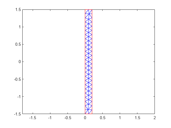

Solve the model and plot the result.

result = solve(thermalmodel);
T = result.Temperature;
figure
pdeplot(thermalmodel,"XYData",T,"Contour","on")
axis equal
title("Steady-State Temperature")

Transient Solution

Switch the analysis type of the model to transient-axisymmetric.

thermalmodel.AnalysisType = "transient-axisymmetric";

Specify the thermal conductivity, mass density, and specific heat of the material.

thermalProperties(thermalmodel,"ThermalConductivity",k,...
                               "MassDensity",rho,...
                               "SpecificHeat",cp);

Specify that the Initial temperature in the rod is 0 °C.

thermalIC(thermalmodel,0);

Compute the transient solution for solution times from t = 0 to t = 50000 seconds.

tfinal = 50000;
tlist = 0:100:tfinal;
result = solve(thermalmodel,tlist);

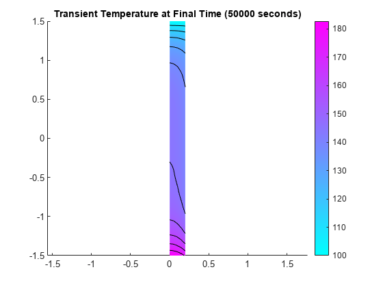
Plot the temperature distribution at t = 50000 seconds.

T = result.Temperature;

figure 
pdeplot(thermalmodel,"XYData",T(:,end),"Contour","on")
axis equal
title(sprintf(['Transient Temperature' ...
               ' at Final Time (%g seconds)'],tfinal))

Find the temperature at the bottom surface of the rod: first, at the center axis and then on the outer surface.

Tcenter = interpolateTemperature(result,[0.0;-1.5],1:numel(tlist));
Touter = interpolateTemperature(result,[0.2;-1.5],1:numel(tlist));

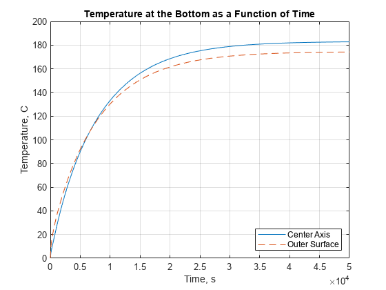
Plot the temperature at the left end of the rod as a function of time. The outer surface of the rod is exposed to the environment with a constant temperature of 100 °C. When the surface temperature of the rod is less than 100 °C, the environment heats the rod. The outer surface is slightly warmer than the inner axis. When the surface temperature is greater than 100 °C, the environment cools the rod. The outer surface becomes cooler than the interior of the rod.

figure
plot(tlist,Tcenter)
hold on
plot(tlist,Touter,"--")
title("Temperature at the Bottom as a Function of Time")
xlabel("Time, s")
ylabel("Temperature, C")
grid on
legend("Center Axis","Outer Surface","Location","SouthEast")