Implement Simultaneous Localization And Mapping (SLAM) with Lidar Scans
This example demonstrates how to implement the Simultaneous Localization And Mapping (SLAM) algorithm on a collected series of lidar scans using pose graph optimization. The goal of this example is to build a map of the environment using the lidar scans and retrieve the trajectory of the robot.
To build the map of the environment, the SLAM algorithm incrementally processes the lidar scans and builds a pose graph that links these scans. The robot recognizes a previously-visited place through scan matching and may establish one or more loop closures along its moving path. The SLAM algorithm utilizes the loop closure information to update the map and adjust the estimated robot trajectory.
Load Laser Scan Data from File
Load a down-sampled data set consisting of laser scans collected from a mobile robot in an indoor environment. The average displacement between every two scans is around 0.6 meters.
The offlineSlamData.mat file contains the scans variable, which contains all the laser scans used in this example.
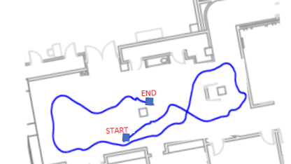
load('offlineSlamData.mat');A floor plan and approximate path of the robot are provided for illustrative purposes. This image shows the relative environment being mapped and the approximate trajectory of the robot.

Run SLAM Algorithm, Construct Optimized Map and Plot Trajectory of the Robot
Create a lidarSLAM object and set the map resolution and the max lidar range. This example uses a Jackal™ robot from Clearpath Robotics™. The robot is equipped with a SICK™ TiM-511 laser scanner with a max range of 10 meters. Set the max lidar range slightly smaller than the max scan range (8m), as the laser readings are less accurate near max range. Set the grid map resolution to 20 cells per meter, which gives a 5cm precision.
maxLidarRange = 8;
mapResolution = 20;
slamAlg = lidarSLAM(mapResolution, maxLidarRange);
The following loop closure parameters are set empirically. Using higher loop closure threshold helps reject false positives in loop closure identification process. However, keep in mind that a high-score match may still be a bad match. For example, scans collected in an environment that has similar or repeated features are more likely to produce false positives. Using a higher loop closure search radius allows the algorithm to search a wider range of the map around current pose estimate for loop closures.
slamAlg.LoopClosureThreshold = 210;
slamAlg.LoopClosureSearchRadius = 8;
Observe the Map Building Process with Initial 10 Scans
Incrementally add scans to the slamAlg object. Scan numbers are printed if added to the map. The object rejects scans if the distance between scans is too small. Add the first 10 scans first to test your algorithm.
for i=1:10
    [isScanAccepted, loopClosureInfo, optimizationInfo] = addScan(slamAlg, scans{i});
    if isScanAccepted
        fprintf('Added scan %d \n', i);
    end
end
Added scan 1
Added scan 2
Added scan 3
Added scan 4
Added scan 5
Added scan 6
Added scan 7
Added scan 8
Added scan 9
Added scan 10
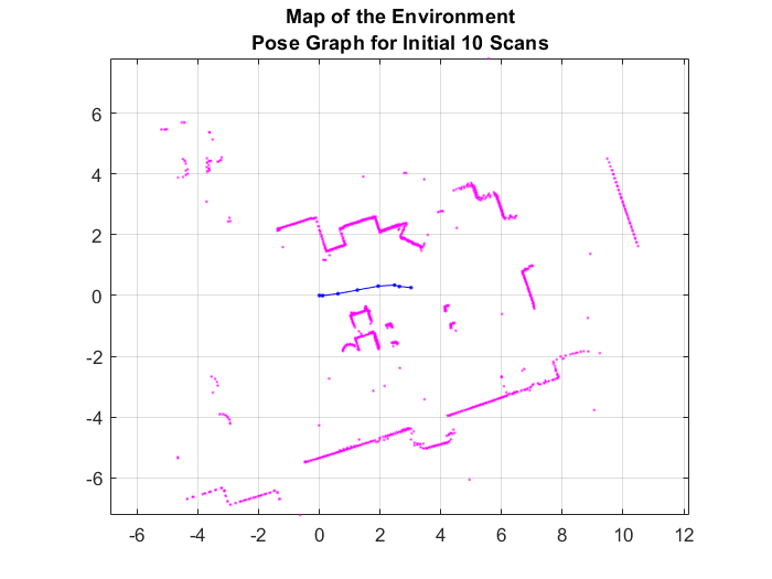
Reconstruct the scene by plotting the scans and poses tracked by the slamAlg.
figure;
show(slamAlg);
title({'Map of the Environment','Pose Graph for Initial 10 Scans'});
Observe the Effect of Loop Closures and the Optimization Process
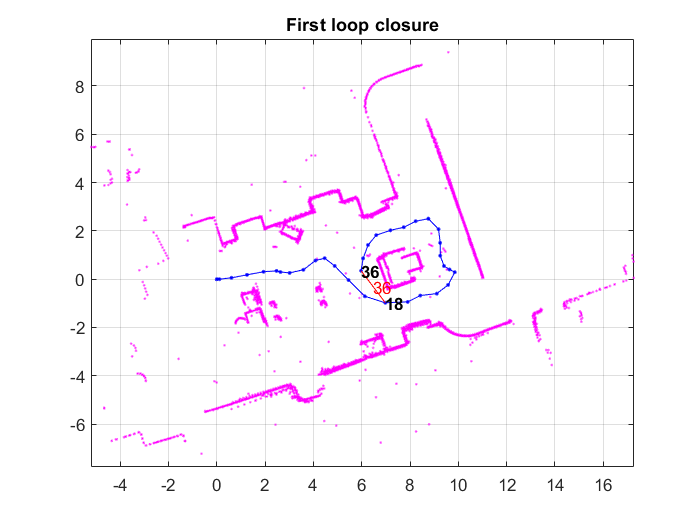
Continue to add scans in a loop. Loop closures should be automatically detected as the robot moves. Pose graph optimization is performed whenever a loop closure is identified. The output optimizationInfo has a field, IsPerformed, that indicates when pose graph optimization occurs.
Plot the scans and poses whenever a loop closure is identified and verify the results visually. This plot shows overlaid scans and an optimized pose graph for the first loop closure. A loop closure edge is added as a red link.
firstTimeLCDetected = false;

figure;
for i=10:length(scans)
    [isScanAccepted, loopClosureInfo, optimizationInfo] = addScan(slamAlg, scans{i});
    if ~isScanAccepted
        continue;
    end
    % visualize the first detected loop closure, if you want to see the
    % complete map building process, remove the if condition below
    if optimizationInfo.IsPerformed && ~firstTimeLCDetected
        show(slamAlg, 'Poses', 'off');
        hold on;
        show(slamAlg.PoseGraph);
        hold off;
        firstTimeLCDetected = true;
        drawnow
    end
end
title('First loop closure');

Visualize the Constructed Map and Trajectory of the Robot
Plot the final built map after all scans are added to the slamAlg object. Though the previous for loop only plotted the initial closure, all the scans were added.
figure
show(slamAlg);
title({'Final Built Map of the Environment', 'Trajectory of the Robot'});
Visually Inspect the Built Map Compared to the Original Floor Plan
An image of the scans and pose graph is overlaid on the original floorplan. You can see that the map matches the original floor plan well after adding all the scans and optimizing the pose graph.

Build Occupancy Grid Map
The optimized scans and poses can be used to generate a occupancyMap, which represents the environment as a probabilistic occupancy grid.
[scans, optimizedPoses]  = scansAndPoses(slamAlg);
map = buildMap(scans, optimizedPoses, mapResolution, maxLidarRange);
Visualize the occupancy grid map populated with the laser scans and the optimized pose graph.
figure;
show(map);
hold on
show(slamAlg.PoseGraph, 'IDs', 'off');
hold off
title('Occupancy Grid Map Built Using Lidar SLAM');

