surrogateopt
Surrogate optimization for global minimization of time-consuming objective functions
Syntax
Description
surrogateopt is a global solver for time-consuming
objective functions.
surrogateopt attempts to solve problems of the form
The solver searches for the global minimum of a real-valued objective function in
multiple dimensions, subject to bounds, optional linear constraints, optional integer
constraints, and optional nonlinear inequality constraints.
surrogateopt is best suited to objective functions that take a
long time to evaluate. The objective function can be nonsmooth. The solver requires
finite bounds on all variables. The solver can optionally maintain a checkpoint file to
enable recovery from crashes or partial execution, or optimization continuation after
meeting a stopping condition. The objective function
f(x) can be empty ([]), in
which case surrogateopt attempts to find a point satisfying all the
constraints.
x = surrogateopt(objconstr,lb,ub)objconstr(x) in the region
lb <= x <= ub. If objconstr(x)
returns a structure, then surrogateopt searches for a
minimum of objconstr(x).Fval, subject to
objconstr(x).Ineq <= 0.
Note
Passing Extra Parameters explains how to pass extra parameters to the objective function, if necessary.
x = surrogateopt(checkpointFile)
x = surrogateopt(checkpointFile,opts)checkpointFile with those in
opts. See Checkpoint File.
Examples
Search for Global Minimum
Search for a minimum of the six-hump camel back function in the region -2.1 <= x(i) <= 2.1. This function has two global minima with the objective function value -1.0316284... and four local minima with higher objective function values.
rng default % For reproducibility objconstr = @(x)(4*x(:,1).^2 - 2.1*x(:,1).^4 + x(:,1).^6/3 ... + x(:,1).*x(:,2) - 4*x(:,2).^2 + 4*x(:,2).^4); lb = [-2.1,-2.1]; ub = -lb; x = surrogateopt(objconstr,lb,ub)
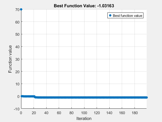
surrogateopt stopped because it exceeded the function evaluation limit set by 'options.MaxFunctionEvaluations'.
x = 1×2
0.0898 -0.7131
Solve Problem with Nonlinear Constraints
Find the minimum of Rosenbrock's function
subject to the nonlinear constraint that the solution lies in a disk of radius 1/3 around the point [1/3,1/3]:
.
To do so, write a function objconstr(x) that returns the value of Rosenbrock's function in a structure field Fval, and returns the nonlinear constraint value in the form in the structure field Ineq.
type objconstrfunction f = objconstr(x) f.Fval = 100*(x(2) - x(1)^2)^2 + (1 - x(1))^2; f.Ineq = (x(1)-1/3)^2 + (x(2)-1/3)^2 - (1/3)^2;
Call surrogateopt using lower bounds of 0 and upper bounds of 2/3 on each component.
lb = [0,0]; ub = [2/3,2/3]; [x,fval,exitflag] = surrogateopt(@objconstr,lb,ub)
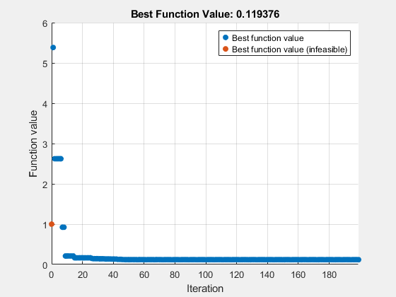
surrogateopt stopped because it exceeded the function evaluation limit set by 'options.MaxFunctionEvaluations'.
x = 1×2
0.6546 0.4277
fval = 0.1194
exitflag = 0
Check the value of the nonlinear constraint at the solution.
disp(objconstr(x).Ineq)
9.9334e-04
The constraint function value is near zero, indicating that the constraint is active at the solution.
Solve Mixed-Integer Problem
Find the minimum of the ps_example function for a two-dimensional variable x whose first component is restricted to integer values, and all components are between –5 and 5.
intcon = 1; rng default % For reproducibility objconstr = @ps_example; lb = [-5,-5]; ub = [5,5]; x = surrogateopt(objconstr,lb,ub,intcon)
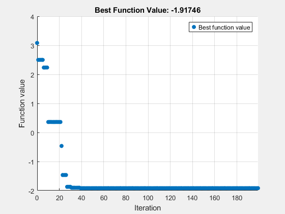
surrogateopt stopped because it exceeded the function evaluation limit set by 'options.MaxFunctionEvaluations'.
x = 1×2
-5.0000 0.0004
Surrogate Optimization Using Nondefault Options
Minimize the six-hump camel back function in the region -2.1 <= x(i) <= 2.1. This function has two global minima with the objective function value -1.0316284... and four local minima with higher objective function values.
To search the region systematically, use a regular grid of starting points. Set 120 as the maximum number of function evaluations. Use the 'surrogateoptplot' plot function. To understand the 'surrogateoptplot' plot, see Interpret surrogateoptplot.
rng default % For reproducibility objconstr = @(x)(4*x(:,1).^2 - 2.1*x(:,1).^4 + x(:,1).^6/3 ... + x(:,1).*x(:,2) - 4*x(:,2).^2 + 4*x(:,2).^4); lb = [-2.1,-2.1]; ub = -lb; [Xpts,Ypts] = meshgrid(-3:3); startpts = [Xpts(:),Ypts(:)]; options = optimoptions('surrogateopt','PlotFcn','surrogateoptplot',... 'InitialPoints',startpts,'MaxFunctionEvaluations',120); x = surrogateopt(objconstr,lb,ub,options)
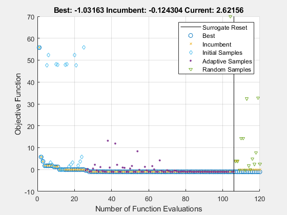
surrogateopt stopped because it exceeded the function evaluation limit set by 'options.MaxFunctionEvaluations'.
x = 1×2
0.0900 -0.7125
Linear Constraints in surrogateopt
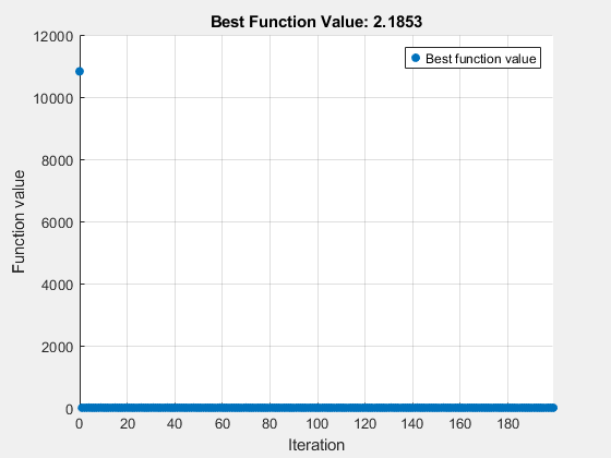
Minimize a nonlinear objective function subject to linear inequality constraints. Minimize for 200 function evaluations.
objconstr = @multirosenbrock; nvar = 6; lb = -2*ones(nvar,1); ub = -lb; intcon = []; A = ones(1,nvar); b = 3; Aeq = []; beq = []; options = optimoptions('surrogateopt','MaxFunctionEvaluations',200); [sol,fval,exitflag,output] = ... surrogateopt(objconstr,lb,ub,intcon,A,b,Aeq,beq,options)
surrogateopt stopped because it exceeded the function evaluation limit set by 'options.MaxFunctionEvaluations'.
sol = 1×6
0.2072 0.0437 0.1360 0.0066 0.1196 -0.0002
fval = 2.1853
exitflag = 0
output = struct with fields:
elapsedtime: 30.0492
funccount: 200
constrviolation: 0
ineq: [1x0 double]
rngstate: [1x1 struct]
message: 'surrogateopt stopped because it exceeded the function evaluation limit set by ...'
Surrogate Optimization of Problem Structure
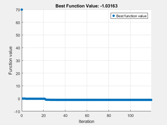
Create a problem structure representing the six-hump camel back function in the region -2.1 <= x(i) <= 2.1. Set 120 as the maximum number of function evaluations.
rng default % For reproducibility objconstr = @(x)(4*x(:,1).^2 - 2.1*x(:,1).^4 + x(:,1).^6/3 ... + x(:,1).*x(:,2) - 4*x(:,2).^2 + 4*x(:,2).^4); options = optimoptions('surrogateopt','MaxFunctionEvaluations',120); problem = struct('objective',objconstr,... 'lb',[-2.1,-2.1],... 'ub',[2.1,2.1],... 'options',options,... 'solver','surrogateopt'); x = surrogateopt(problem)
surrogateopt stopped because it exceeded the function evaluation limit set by 'options.MaxFunctionEvaluations'.
x = 1×2
0.0898 -0.7131
Return Surrogate Optimization Objective Function Value
Minimize the six-hump camel back function and return both the minimizing point and the objective function value. Set options to suppress all other display.
rng default % For reproducibility objconstr = @(x)(4*x(:,1).^2 - 2.1*x(:,1).^4 + x(:,1).^6/3 ... + x(:,1).*x(:,2) - 4*x(:,2).^2 + 4*x(:,2).^4); lb = [-2.1,-2.1]; ub = -lb; options = optimoptions('surrogateopt','Display','off','PlotFcn',[]); [x,fval] = surrogateopt(objconstr,lb,ub,options)
x = 1×2
0.0898 -0.7131
fval = -1.0316
Monitor Surrogate Optimization Process
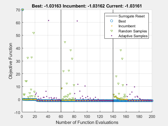
Monitor the surrogate optimization process by requesting that surrogateopt return more outputs. Use the 'surrogateoptplot' plot function. To understand the 'surrogateoptplot' plot, see Interpret surrogateoptplot.
rng default % For reproducibility objconstr = @(x)(4*x(:,1).^2 - 2.1*x(:,1).^4 + x(:,1).^6/3 ... + x(:,1).*x(:,2) - 4*x(:,2).^2 + 4*x(:,2).^4); lb = [-2.1,-2.1]; ub = -lb; options = optimoptions('surrogateopt','PlotFcn','surrogateoptplot'); [x,fval,exitflag,output] = surrogateopt(objconstr,lb,ub,options)
surrogateopt stopped because it exceeded the function evaluation limit set by 'options.MaxFunctionEvaluations'.
x = 1×2
0.0898 -0.7131
fval = -1.0316
exitflag = 0
output = struct with fields:
elapsedtime: 12.2933
funccount: 200
constrviolation: 0
ineq: [1x0 double]
rngstate: [1x1 struct]
message: 'surrogateopt stopped because it exceeded the function evaluation limit set by ...'
Restart Surrogate Optimization
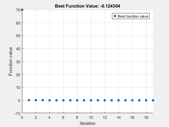
Conclude a surrogate optimization quickly by setting a small maximum number of function evaluations. To prepare for the possibility of restarting the optimization, request all solver outputs.
rng default % For reproducibility objconstr = @(x)(4*x(:,1).^2 - 2.1*x(:,1).^4 + x(:,1).^6/3 ... + x(:,1).*x(:,2) - 4*x(:,2).^2 + 4*x(:,2).^4); lb = [-2.1,-2.1]; ub = -lb; options = optimoptions('surrogateopt','MaxFunctionEvaluations',20); [x,fval,exitflag,output,trials] = surrogateopt(objconstr,lb,ub,options);
surrogateopt stopped because it exceeded the function evaluation limit set by 'options.MaxFunctionEvaluations'.
Optimize for another 20 function evaluations, starting from the previously evaluated points.
options.InitialPoints = trials; [x,fval,exitflag,output,trials] = surrogateopt(objconstr,lb,ub,options);
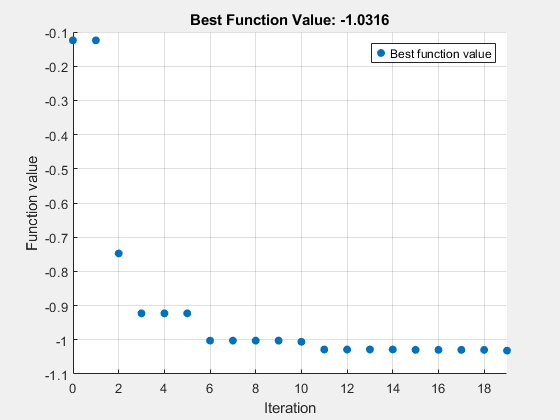
surrogateopt stopped because it exceeded the function evaluation limit set by 'options.MaxFunctionEvaluations'.
By comparing the plots of these 40 function evaluations to those in Search for Global Minimum, you see that restarting surrogate optimization is not the same as having the solver run continuously.
Restart Surrogate Optimization from Checkpoint File
To enable restarting surrogate optimization due to a crash or any other reason, set a checkpoint file name.
opts = optimoptions('surrogateopt','CheckpointFile','checkfile.mat');
Create an optimization problem and set a small number of function evaluations.
rng default % For reproducibility objconstr = @(x)(4*x(:,1).^2 - 2.1*x(:,1).^4 + x(:,1).^6/3 ... + x(:,1).*x(:,2) - 4*x(:,2).^2 + 4*x(:,2).^4); lb = [-2.1,-2.1]; ub = -lb; opts.MaxFunctionEvaluations = 30; [x,fval,exitflag,output] = surrogateopt(objconstr,lb,ub,opts)

Surrogateopt stopped because it exceeded the function evaluation limit set by 'options.MaxFunctionEvaluations'.
x = 1×2
0.0067 -0.7343
fval = -0.9986
exitflag = 0
output = struct with fields:
elapsedtime: 28.7221
funccount: 30
constrviolation: 0
ineq: [1×0 double]
rngstate: [1×1 struct]
message: 'Surrogateopt stopped because it exceeded the function evaluation limit set by ↵'options.MaxFunctionEvaluations'.'
Set options to use 100 function evaluations (which means 70 more than already done) and restart the optimization.
opts.MaxFunctionEvaluations = 100;
[x2,fval2,exitflag2,output2] = surrogateopt('checkfile.mat',opts)
Surrogateopt stopped because it exceeded the function evaluation limit set by 'options.MaxFunctionEvaluations'.
x2 = 1×2
0.0895 -0.7130
fval2 = -1.0316
exitflag2 = 0
output2 = struct with fields:
elapsedtime: 159.2411
funccount: 100
constrviolation: 0
ineq: [1×0 double]
rngstate: [1×1 struct]
message: 'Surrogateopt stopped because it exceeded the function evaluation limit set by ↵'options.MaxFunctionEvaluations'.'
Input Arguments
objconstr — Objective function and nonlinear constraint
function handle | function name
Objective function and nonlinear constraint, specified as a function
handle or function name. objconstr accepts a single
argument x, where x is typically a row
vector. However, when the Vectorized option is
true, x is a matrix containing
options.BatchUpdateInterval rows; each row represents
one point to evaluate. objconstr returns one of the
following:
Real scalar
fval = objconstr(x).Structure. If the structure contains the field
Fval, thensurrogateoptattempts to minimizeobjconstr(x).Fval. If the structure contains the fieldIneq, thensurrogateoptattempts to make all components of that field nonpositive:objconstr(x).Ineq <= 0for all entries.objconstr(x)must include either theFvalorIneqfields, or both.surrogateoptignores other fields.
When the Vectorized option is true
and the BatchUpdateInterval is greater than one,
objconstr operates on each row of
x and returns one of the following:
Real vector
fval = objconstr(x).fvalis a column vector withoptions.BatchUpdateIntervalentries (or fewer for the last function evaluation whenBatchUpdateIntervaldoes not evenly divideMaxFunctionEvaluations).Structure with vector entries. If the structure contains the field
Fval, thensurrogateoptattempts to minimizeobjconstr(x).Fval, andobjconstr(x).Fvalis a vector of lengthBatchUpdateInterval(or less). If the structure contains the fieldIneq, thensurrogateoptattempts to make all components of that field nonpositive:objconstr(x).Ineq <= 0for all entries, andobjconstr(x).Ineqcontains up toBatchUpdateIntervalentries.
The objective function objconstr.Fval can be empty
([]), in which case surrogateopt
attempts to find a point satisfying all the constraints. See Solve Feasibility Problem.
For examples using a nonlinear constraint, see Solve Problem with Nonlinear Constraints, Surrogate Optimization with Nonlinear Constraint, and Solve Feasibility Problem. For
information on converting between the surrogateopt
structure syntax and other solvers, see packfcn and Convert Nonlinear Constraints Between surrogateopt Form and Other Solver Forms For an
example using vectorized batch evaluations, see Optimize Simulink Model in Parallel.
Data Types: function_handle | char | string
lb — Lower bounds
finite real vector
Lower bounds, specified as a finite real vector. lb
represents the lower bounds element-wise in
lb ≤ x ≤ ub.
The lengths of lb and ub must be equal
to the number of variables that objconstr
accepts.
Caution
Although lb is optional for most solvers,
lb is a required input for
surrogateopt.
Note
surrogateopt allows equal entries in lb and
ub. For each i in intcon, you
must have ceil(lb(i)) <= floor(ub(i)). See Construct Surrogate Details.
Example: lb = [0;-20;4] means x(1) ≥
0, x(2) ≥ -20, x(3) ≥
4.
Data Types: double
ub — Upper bounds
finite real vector
Upper bounds, specified as a finite real vector. ub
represents the upper bounds element-wise in
lb ≤ x ≤ ub.
The lengths of lb and ub must be equal
to the number of variables that objconstr
accepts.
Caution
Although ub is optional for most solvers,
ub is a required input for
surrogateopt.
Note
surrogateopt allows equal entries in lb and
ub. For each i in intcon, you
must have ceil(lb(i)) <= floor(ub(i)). See Construct Surrogate Details.
Example: ub = [10;-20;4] means x(1) ≤
10, x(2) ≤ -20, x(3) ≤
4.
Data Types: double
intcon — Integer variables
vector of positive integers
Integer variables, specified as a vector of positive integers with values
from 1 to the number of problem variables. Each value in
intcon represents an x component
that is integer-valued.
Example: To specify that the even entries in x are
integer-valued, set intcon to
2:2:nvars.
Data Types: double
A — Linear inequality constraints
real matrix
Linear inequality constraints, specified as a real matrix. A is an M-by-nvars matrix, where M is the number of inequalities.
A encodes the M linear inequalities
A*x <= b,
where x is the column vector of nvars variables x(:), and b is a column vector with M elements.
For example, to specify
x1 + 2x2 ≤ 10
3x1 + 4x2 ≤ 20
5x1 + 6x2 ≤ 30,
give these constraints:
A = [1,2;3,4;5,6]; b = [10;20;30];
Example: To specify that the control variables sum to 1 or less, give the constraints
A = ones(1,N) and b = 1.
Data Types: double
b — Linear inequality constraints
real vector
Linear inequality constraints, specified as a real vector. b is an M-element vector related to the A matrix. If you pass b as a row vector, solvers internally convert b to the column vector b(:).
b encodes the M linear inequalities
A*x <= b,
where x is the column vector of N variables x(:), and A is a matrix of size M-by-N.
For example, to specify
x1 + 2x2 ≤ 10
3x1 + 4x2 ≤ 20
5x1 + 6x2 ≤ 30,
give these constraints:
A = [1,2;3,4;5,6]; b = [10;20;30];
Example: To specify that the control variables sum to 1 or less, give the constraints
A = ones(1,N) and b = 1.
Data Types: double
Aeq — Linear equality constraints
real matrix
Linear equality constraints, specified as a real matrix. Aeq is an Me-by-nvars matrix, where Me is the number of equalities.
Aeq encodes the Me linear equalities
Aeq*x = beq,
where x is the column vector of N variables x(:), and beq is a column vector with Me elements.
For example, to specify
x1
+ 2x2 +
3x3 =
10
2x1
+ 4x2 +
x3 =
20,
give these constraints:
Aeq = [1,2,3;2,4,1];
beq = [10;20];
Example: To specify that the control variables sum to 1, give the constraints Aeq =
ones(1,N) and beq = 1.
Data Types: double
beq — Linear equality constraints
real vector
Linear equality constraints, specified as a real vector. beq is an Me-element vector related to the Aeq matrix. If you pass beq as a row vector, solvers internally convert beq to the column vector beq(:).
beq encodes the Me linear equalities
Aeq*x = beq,
where x is the column vector of N variables x(:), and Aeq is a matrix of size Meq-by-N.
For example, to specify
x1
+ 2x2 +
3x3 =
10
2x1
+ 4x2 +
x3 =
20,
give these constraints:
Aeq = [1,2,3;2,4,1];
beq = [10;20];
Example: To specify that the control variables sum to 1, give the constraints Aeq =
ones(1,N) and beq = 1.
Data Types: double
options — Options
output of optimoptions
Options, specified as the output of
optimoptions.
For more information, see Surrogate Optimization Options.
| Option | Description | Values |
|---|---|---|
BatchUpdateInterval |
| Positive integer. Default is
|
CheckpointFile | File name for checkpointing and restarting
optimization. The file has the Checkpointing takes time. This overhead is especially noticeable for functions that otherwise take little time to evaluate. | File name or file path, given as a string or
character array. If you specify a file name without a
path, |
ConstraintTolerance | Tolerance on nonlinear constraints, measured as the maximum of all nonlinear constraint function values, where positive values indicate a violation. This tolerance is an absolute (not relative) tolerance; see Tolerances and Stopping Criteria. | Nonnegative scalar. Default is
1e-3. |
Display | Level of display returned at the command line. |
|
InitialPoints | Initial points for solver. | Matrix of initial points, where each row is one
point. Or, a structure with field
See Algorithm Control. Default is |
MaxFunctionEvaluations | Maximum number of objective function evaluations, a stopping criterion. | Nonnegative integer. Default is
max(200,50*nvar), where
nvar is the number of problem
variables. |
MaxTime | Maximum running time in seconds. The actual running time
can exceed MaxTime because of the time
required to evaluate an objective function or because of
parallel processing delays. | Nonnegative scalar. Default is
Inf. |
MinSampleDistance | Minimum distance between trial points generated by the adaptive sampler. See Surrogate Optimization Algorithm. | Nonnegative scalar. Default is
1e-6. |
MinSurrogatePoints | Minimum number of random sample points to create at the start of a surrogate creation phase. See Surrogate Optimization Algorithm. When | Integer at least nvar + 1. Default is
max(20,2*nvar), where
nvar is the number of problem
variables. |
ObjectiveLimit | Tolerance on the objective function value. If a
calculated objective function value of a feasible point is
less than ObjectiveLimit, the algorithm
stops. | Double scalar value. Default is
-Inf. |
OutputFcn | Output function to report on solver progress or to stop the solver. See Output Function. | Function name, function handle, or cell array of function
names or handles. Default is []. |
PlotFcn | Plot function to display solver progress or to stop solver. See Plot Function. | Function name, function handle, or cell array of function names or handles. Built-in plot functions are:
|
UseParallel | Boolean value indicating whether to compute objective function values in parallel. You cannot specify both | Boolean. Default is false. For
algorithmic details, see Parallel surrogateopt Algorithm. |
UseVectorized | Boolean value indicating whether to compute
objective function values in batches of size
You cannot specify both | Boolean. Default is false. For an
example, see Optimize Simulink Model in Parallel. |
Example: options =
optimoptions('surrogateopt','Display','iter','UseParallel',true)
problem — Problem structure
structure
Problem structure, specified as a structure with these fields:
objective— Objective function, which can include nonlinear constraints, specified as a function name or function handlelb— Lower bounds forxub— Upper bounds forxsolver—'surrogateopt'Aineq— Matrix for linear inequality constraints (optional)bineq— Vector for linear inequality constraints (optional)Aeq— Matrix for linear equality constraints (optional)beq— Vector for linear equality constraints (optional)options— Options created withoptimoptionsrngstate— Field to reset the state of the random number generator (optional)intcon— Field specifying integer-valuedxcomponents (optional)
Note
These problem fields are required:
objective, lb,
ub, solver, and
options.
Data Types: struct
checkpointFile — Path to checkpoint file
string | character vector
Path to a checkpoint file, specified as a string or character vector. A
checkpoint file has the .mat extension. If you specify a
file name without a path, surrogateopt uses a checkpoint
file in the current folder.
A checkpoint file stores the state of an optimization for resuming the
optimization. surrogateopt updates the checkpoint file
at each function evaluation, so you can resume the optimization even when
surrogateopt halts prematurely. For an example, see
Restart Surrogate Optimization from Checkpoint File.
surrogateopt creates a checkpoint file when it has a
valid CheckpointFile option.
You can change some options when resuming from a checkpoint file. See
opts.
The data in a checkpoint file is in .mat format. To
avoid errors or other unexpected results, do not modify the data before
calling surrogateopt.
Warning
Do not resume surrogateopt from a checkpoint file created with a
different MATLAB® version. surrogateopt can throw an error or give
inconsistent results.
Example: 'checkfile.mat'
Example: "C:\Program
Files\MATLAB\docs\checkpointNov2019.mat"
Data Types: char | string
opts — Options for resuming from checkpoint file
[] (default) | optimoptions options from a restricted set
Options for resuming optimization from the checkpoint file, specified as
optimoptions options (from a restricted set) that you
can change from the original options. The options you can change are:
BatchUpdateIntervalCheckpointFileDisplayMaxFunctionEvaluationsMaxTimeMinSurrogatePointsObjectiveLimitOutputFcnPlotFcnUseParallelUseVectorized
Example: opts =
optimoptions(options,'MaxFunctionEvaluations',400);
Output Arguments
fval — Objective function value at solution
real number
exitflag — Reason surrogateopt stopped
integer
Reason surrogateopt stopped, returned as one of the
integer values described in this table.
| Exit Flag | Description |
|---|---|
| Problem has a unique feasible solution due to one of the following:
|
3 | Feasible point found. Solver stopped because too few new feasible points were found to continue. |
| The objective function value is less than
|
| The number of function evaluations exceeds
|
| The optimization is terminated by an output function or plot function. |
| No feasible point is found due to one of the following:
|
output — Information about optimization process
structure
Information about the optimization process, returned as a structure with these fields:
funccount— Total number of function evaluations.elapsedtime— Time spent running the solver in seconds, as measured bytic/toc.message— Reason why the algorithm stopped.constrviolation— Maximum nonlinear constraint violation, if any.constrviolation = max(output.ineq).ineq— Nonlinear inequality constraint value at the solutionx. Ifobjconstrreturns a structure, thenineq=objconstr(x).Ineq. Otherwise,ineqis empty.rngstate— State of the MATLAB random number generator just before the algorithm starts. Use this field to reproduce your results. See Reproduce Results, which discusses usingrngstateforga.
trials — Points evaluated
structure
Points evaluated, returned as a structure with these fields:
X— Matrix withnvarscolumns, wherenvarsis the length oflborub. Each row ofXrepresents one point evaluated bysurrogateopt.Fval— Column vector, where each entry is the objective function value of the corresponding row ofX.Ineq— Matrix with each row representing the constraint function values of the corresponding row ofX.
The trials structure has the same form as the
options.InitialPoints structure. So, you can continue
an optimization by passing the trials structure as the
InitialPoints option.
Algorithms
surrogateopt repeatedly performs these steps:
Create a set of trial points by sampling
MinSurrogatePointsrandom points within the bounds, and evaluate the objective function at the trial points.Create a surrogate model of the objective function by interpolating a radial basis function through all of the random trial points.
Create a merit function that gives some weight to the surrogate and some weight to the distance from the trial points. Locate a small value of the merit function by randomly sampling the merit function in a region around the incumbent point (best point found since the last surrogate reset). Use this point, called the adaptive point, as a new trial point.
Evaluate the objective at the adaptive point, and update the surrogate based on this point and its value. Count a "success" if the objective function value is sufficiently lower than the previous best (lowest) value observed, and count a "failure" otherwise.
Update the dispersion of the sample distribution upwards if three successes occur before
max(nvar,5)failures, wherenvaris the number of dimensions. Update the dispersion downwards ifmax(nvar,5)failures occur before three successes.Continue from step 3 until all trial points are within
MinSampleDistanceof the evaluated points. At that time, reset the surrogate by discarding all adaptive points from the surrogate, reset the scale, and go back to step 1 to createMinSurrogatePointsnew random trial points for evaluation.
For details, see Surrogate Optimization Algorithm.
Alternative Functionality
App
The Optimize Live Editor task provides a visual interface for surrogateopt.
Extended Capabilities
Automatic Parallel Support
Accelerate code by automatically running computation in parallel using Parallel Computing Toolbox™.
To run in parallel, set the 'UseParallel' option to true.
options = optimoptions('solvername','UseParallel',true)
For more information, see How to Use Parallel Processing in Global Optimization Toolbox.
Version History
Introduced in R2018bR2024a: surrogateopt algorithm efficiency improved
surrogateopt has updated internal routines that increase its
efficiency, especially for integer-constrained problems. Also, for problems with
fast objective and nonlinear constraint functions, checkpointing is more efficient
than before: surrogateopt writes checkpoint files no more than
once in 10 seconds. For details, see Surrogate Optimization Algorithm and Checkpoint File.
MATLAB Command
You clicked a link that corresponds to this MATLAB command:
Run the command by entering it in the MATLAB Command Window. Web browsers do not support MATLAB commands.

Select a Web Site
Choose a web site to get translated content where available and see local events and offers. Based on your location, we recommend that you select: .
You can also select a web site from the following list
How to Get Best Site Performance
Select the China site (in Chinese or English) for best site performance. Other bat365 country sites are not optimized for visits from your location.
Americas
- América Latina (Español)
- Canada (English)
- United States (English)
Europe
- Belgium (English)
- Denmark (English)
- Deutschland (Deutsch)
- España (Español)
- Finland (English)
- France (Français)
- Ireland (English)
- Italia (Italiano)
- Luxembourg (English)
- Netherlands (English)
- Norway (English)
- Österreich (Deutsch)
- Portugal (English)
- Sweden (English)
- Switzerland
- United Kingdom (English)
Asia Pacific
- Australia (English)
- India (English)
- New Zealand (English)
- 中国
- 日本Japanese (日本語)
- 한국Korean (한국어)