Exposures Simulation

Many financial institutions have systems that simulate market risk factors and value all the instruments in their portfolios at given simulation dates. These simulations are used to compute exposures and other risk measures. Because the simulations are computationally intensive, reusing them for subsequent risk analyses is important.

This example uses the data and the simulation results from the Counterparty Credit Risk and CVA example, previously saved in the ccr.mat file. The ccr.mat file contains:

This example looks at expected losses over a one-year time horizon only, so the data is cropped after one year of simulation. Simulation dates over the first year are at a monthly frequency, so the 13th simulation date is our one-year time horizon (the first simulation date is the settle date).

load ccr.mat

oneYearIdx = 13;
values = values(1:oneYearIdx,:,:);
dates = simulationDates(1:oneYearIdx);

numScenarios = size(values,3);

The credit exposures are computed from the simulated contract values. These exposures are monthly credit exposures per counterparty from the settle date to our one-year time horizon.

Since defaults can happen at any time during the one-year time period, it is common to model the exposure at default (EAD) based on the idea of expected positive exposure (EPE). The time-averaged exposure for each scenario is computed, which is called PE (positive exposure). The average of the PE's, including all scenarios, is the EPE, which can also be obtained from the exposureprofiles function.

The positive exposure matrix PE contains one row per simulated scenario and one column per counterparty. This is used as the EAD in this analysis.

% Compute counterparty exposures
[exposures, counterparties] = creditexposures(values,swaps.Counterparty, ...
    'NettingID',swaps.NettingID);
numCP = numel(counterparties);

% Compute PE (time-averaged exposures) per scenario
intervalWeights = diff(dates) / (dates(end) - dates(1));
exposureMidpoints = 0.5 * (exposures(1:end-1,:,:) + exposures(2:end,:,:));
weightedContributions = bsxfun(@times,intervalWeights,exposureMidpoints);
PE = squeeze(sum(weightedContributions))';

% Compute total portfolio exposure per scenario
totalExp = sum(PE,2);

% Display size of PE and totalExp
whos PE totalExp

  Name             Size            Bytes  Class     Attributes

  PE            1000x5             40000  double              
  totalExp      1000x1              8000  double              

Credit Simulation

A common approach for simulating credit defaults is based on a "one-factor model", sometimes called the "asset-value approach" (see Gupton et al., 1997). This is an efficient way to simulate correlated defaults.

Each company i is associated with a random variable Yi, such that

where Z is the "one-factor", a standard normal random variable that represents a systematic credit risk factor whose values affect all companies. The correlation between company i and the common factor is given by beta_i, the correlation between companies i and j is beta_i*beta_j. The idiosyncratic shock epsilon_i is another standard normal variable that may reduce or increase the effect of the systematic factor, independently of what happens with any other company.

If the default probability for company i is PDi, a default occurs when

where $$\Phi$$ is the cumulative standard normal distribution.

The Yi variable is sometimes interpreted as asset returns, or sometimes referred to as a latent variable.

This model is a Gaussian copula that introduces a correlation between credit defaults. Copulas offer a particular way to introduce correlation, or more generally, co-dependence between two random variables whose co-dependence is unknown.

Use CDS spreads to bootstrap the one-year default probabilities for each counterparty. The CDS quotes come from the swap-portfolio spreadsheet used in the Counterparty Credit Risk and CVA example.

% Import CDS market information for each counterparty
swapFile = 'cva-swap-portfolio.xls';
cds = readtable(swapFile,'Sheet','CDS Spreads');
cdsDates = datenum(cds.Date);
cdsSpreads = table2array(cds(:,2:end));

% Bootstrap default probabilities for each counterparty
zeroData = [RateSpec.EndDates RateSpec.Rates];
defProb = zeros(1, size(cdsSpreads,2));
for i = 1:numel(defProb)
    probData = cdsbootstrap(zeroData, [cdsDates cdsSpreads(:,i)], ...
        Settle, 'probDates', dates(end));
    defProb(i) = probData(2);
end

Now simulate the credit scenarios. Because defaults are rare, it is common to simulate a large number of credit scenarios.

The sensitivity parameter beta is set to 0.3 for all counterparties. This value can be calibrated or tuned to explore model sensitivities. See the References for more information.

numCreditScen = 100000;
rng('default');

% Z is the single credit factor
Z = randn(numCreditScen,1);

% epsilon is the idiosyncratic factor
epsilon = randn(numCreditScen,numCP);

% beta is the counterparty sensitivity to the credit factor
beta = 0.3 * ones(1,numCP);

% Counterparty latent variables
Y = bsxfun(@times,beta,Z) + bsxfun(@times,sqrt(1 - beta.^2),epsilon);

% Default indicator
isDefault = bsxfun(@lt,normcdf(Y),defProb);

Correlating Exposure and Credit Scenarios

Now that there is a set of sorted portfolio exposure scenarios and a set of default scenarios, follow the approach in Garcia Cespedes et al. and use a Gaussian copula to generate correlated exposure-default scenario pairs.

Define a latent variable Ye that maps into the distribution of simulated exposures. Ye is defined as

where Z is the systemic factor computed in the credit simulation, epsilon_e is an independent standard normal variable and rho is interpreted as a market-credit correlation parameter. By construction, Ye is a standard normal variable correlated with Z with correlation parameter rho.

The mapping between Ye and the simulated exposures requires us to order the exposure scenarios in a meaningful way, based on some sortable criterion. The criterion can be any meaningful quantity, for example, it could be an underlying risk factor for the contract values (such as an interest rate), the total portfolio exposure, and so on.

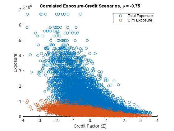
In this example, use the total portfolio exposure (totalExp) as the exposure scenario criterion to correlate the credit factor with the total exposure. If rho is negative, low values of the credit factor Z tend to get linked to high values of Ye, hence high exposures. This means negative values of rho introduce WWR.

To implement the mapping between Ye and the exposure scenarios, sort the exposure scenarios by the totalExp values. Suppose that the number of exposure scenarios is S (numScenarios). Given Ye, find the value j such that

and select the scenario j from the sorted exposure scenarios.

Ye is correlated to the simulated exposures and Z is correlated to the simulated defaults. The correlation rho between Ye and Z is, therefore, the correlation link between the exposures and the credit simulations.

% Sort the total exposure
[~,totalExpIdx] = sort(totalExp);

% Scenario cut points
cutPoints = 0:1/numScenarios:1;

% epsilonExp is the idiosyncratic factor for the latent variable
epsilonExp = randn(numCreditScen,1);

% Set a market-credit correlation value
rho = -0.75;

% Latent variable
Ye = rho * Z + sqrt(1 - rho^2) * epsilonExp;

% Find corresponding exposure scenario
binidx = discretize(normcdf(Ye),cutPoints);
scenIdx = totalExpIdx(binidx);
totalExpCorr = totalExp(scenIdx);
PECorr = PE(scenIdx,:);

The following plot shows the correlated exposure-credit scenarios for the total portfolio exposure as well as for the first counterparty. Because of the negative correlation, negative values of the credit factor Z correspond to high exposure levels (wrong-way risk).

% We only plot up to 10000 scenarios
numScenPlot = min(10000,numCreditScen);
figure;
scatter(Z(1:numScenPlot),totalExpCorr(1:numScenPlot))
hold on
scatter(Z(1:numScenPlot),PECorr(1:numScenPlot,1))
xlabel('Credit Factor (Z)')
ylabel('Exposure')
title(['Correlated Exposure-Credit Scenarios, \rho = ' num2str(rho)])
legend('Total Exposure','CP1 Exposure')
hold off

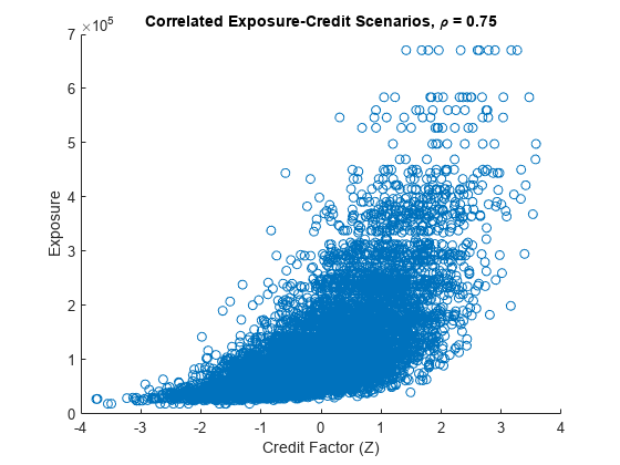
For positive values of rho, the relationship between the credit factor and the exposures is reversed (right-way risk).

rho = 0.75;
Ye = rho * Z + sqrt(1 - rho^2) * epsilonExp;
binidx = discretize(normcdf(Ye),cutPoints);
scenIdx = totalExpIdx(binidx);
totalExpCorr = totalExp(scenIdx);

figure;
scatter(Z(1:numScenPlot),totalExpCorr(1:numScenPlot))
xlabel('Credit Factor (Z)')
ylabel('Exposure')
title(['Correlated Exposure-Credit Scenarios, \rho = ' num2str(rho)])

Sensitivity to Correlation

You can explore the sensitivity of the exposures or other risk measures to a range of values for rho.

For each value of rho, compute the total losses per credit scenario as well as the expected losses per counterparty. This example assumes a 40% recovery rate.

Recovery = 0.4;
rhoValues = -1:0.1:1;

totalLosses = zeros(numCreditScen,numel(rhoValues));
expectedLosses = zeros(numCP, numel(rhoValues));

for i = 1:numel(rhoValues)
    
    rho = rhoValues(i);
    
    % Latent variable
    Ye = rho * Z + sqrt(1 - rho^2) * epsilonExp;
    
    % Find corresponding exposure scenario
    binidx = discretize(normcdf(Ye),cutPoints);
    scenIdx = totalExpIdx(binidx);
    simulatedExposures = PE(scenIdx,:);
    
    % Compute actual losses based on exposures and default events
    losses = isDefault .* simulatedExposures * (1-Recovery);    
    totalLosses(:,i) = sum(losses,2);
    
    % We compute the expected losses per counterparty
    expectedLosses(:,i) = mean(losses)';    
end
displayExpectedLosses(rhoValues, expectedLosses)

               Expected Losses
 Rho    CP1      CP2      CP3     CP4       CP5
-------------------------------------------------
-1.0   604.10   260.44   194.70  1234.17   925.95-0.9   583.67   250.45   189.02  1158.65   897.91-0.8   560.45   245.19   183.23  1107.56   865.33-0.7   541.08   235.86   177.16  1041.39   835.12-0.6   521.89   228.78   170.49   991.70   803.22-0.5   502.68   217.30   165.25   926.92   774.27-0.4   487.15   211.29   160.80   881.03   746.15-0.3   471.17   203.55   154.79   828.90   715.63-0.2   450.91   197.53   149.33   781.81   688.13-0.1   433.87   189.75   144.37   744.00   658.19 0.0   419.20   181.25   138.76   693.26   630.38 0.1   399.36   174.41   134.83   650.66   605.89 0.2   385.21   169.86   130.93   617.91   579.01 0.3   371.21   164.19   124.62   565.78   552.83 0.4   355.57   158.14   119.92   530.79   530.19 0.5   342.58   152.10   116.38   496.27   508.86 0.6   324.73   145.42   111.90   466.57   485.05 0.7   319.18   140.76   108.14   429.48   465.84 0.8   303.71   136.13   103.95   405.88   446.36 0.9   290.36   131.54   100.20   381.27   422.79 1.0   278.89   126.77    95.77   358.71   405.40

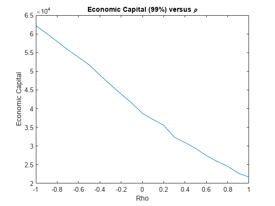
You can visualize the sensitivity of the Economic Capital (EC) to the market-credit correlation parameter. Define EC as the difference between a percentile q of the distribution of losses, minus the expected loss.

Negative values of rho result in higher capital requirements because of WWR.

pct = 99;
ec = prctile(totalLosses,pct) - mean(totalLosses);

figure;
plot(rhoValues,ec)
title('Economic Capital (99%) versus \rho')
xlabel('Rho');
ylabel('Economic Capital');

Final Remarks

This example implements a copula-based approach to WWR, following Garcia Cespedes et al. The methodology can efficiently reuse existing exposures and credit simulations, and the sensitivity to the market-credit correlation parameter can be efficiently computed and conveniently visualized for all correlation values.

The single-parameter copula approach presented here can be extended for a more thorough exploration of the WWR of a portfolio. For example, different types of copulas can be applied, and different criteria can be used to sort the exposure scenarios. Other extensions include simulating multiple systemic credit risk variables (a multi-factor model), or switching from a one-year to a multi-period framework to calculate measures such as credit value adjustment (CVA), as in Rosen and Saunders (see References).

References

Local Functions

function displayExpectedLosses(rhoValues, expectedLosses)
fprintf('               Expected Losses\n');
fprintf(' Rho    CP1      CP2      CP3     CP4       CP5\n');
fprintf('-------------------------------------------------\n');
for i = 1:numel(rhoValues)
    % Display expected loss
    fprintf('% .1f%9.2f%9.2f%9.2f%9.2f%9.2f', rhoValues(i), expectedLosses(:,i));  
end
end

References

Garcia Cespedes, J. C. "Effective Modeling of Wrong-Way Risk, Counterparty Credit Risk Capital, and Alpha in Basel II." The Journal of Risk Model Validation, Volume 4 / Number 1, pp. 71-98, Spring 2010.
Gupton, G., C. Finger, and M. Bathia. CreditMetrics™ - Technical Document. J.P. Morgan, New York, 1997.
Rosen, D., and D. Saunders. "CVA the Wrong Way." Journal of Risk Management in Financial Institutions. Vol. 5, No. 3, pp. 252-272, 2012.