Price Swaptions with Negative Strikes Using the Shifted SABR Model
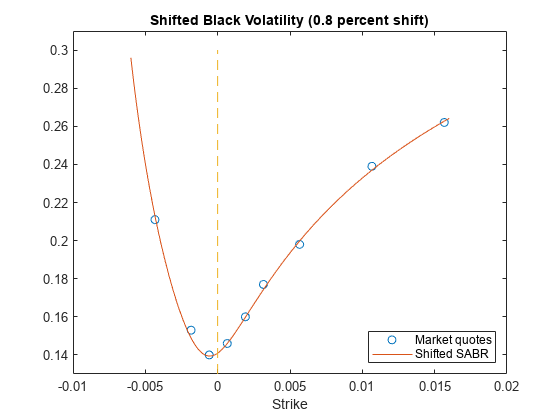
This example shows how to price swaptions with negative strikes by using the Shifted SABR model. The market Shifted Black volatilities are used to calibrate the Shifted SABR model parameters. The calibrated Shifted SABR model is then used to compute the Shifted Black volatilities for negative strikes.
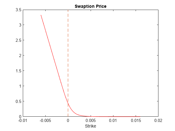
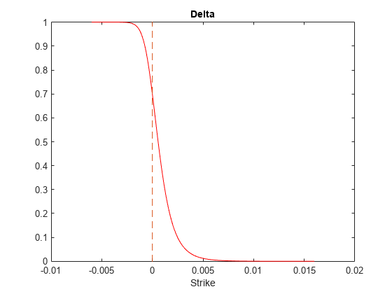
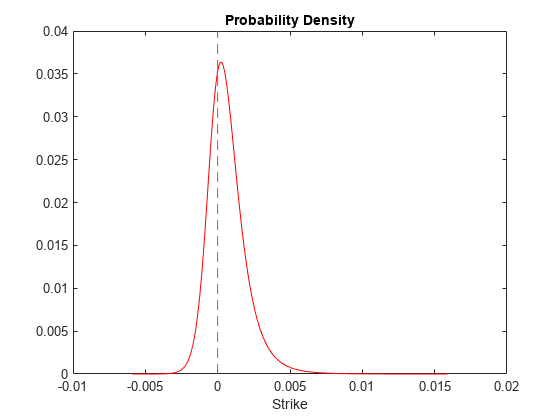
The swaptions with negative strikes are then priced using the computed Shifted Black volatilities and the swaptionbyblk function with the 'Shift' parameter set to the prespecified shift. Similarly, Shifted SABR Greeks can be computed by using the optsensbysabr function by setting the 'Shift' parameter. Finally, from the swaption prices, the probability density of the underlying asset is computed to show that the swaption prices imply positive probability densities for some negative strikes.
Load the market data.
First, load the market interest rates and swaption volatility data. The market swaption volatilities are quoted in terms of Shifted Black volatilities with a 0.8 percent shift.
Define RateSpec.
ValuationDate = '5-Apr-2016';
EndDates = datemnth(ValuationDate,[1 2 3 6 9 12*[1 2 3 4 5 6 7 8 9 10 12]])';
ZeroRates = [-0.34 -0.29 -0.25 -0.13 -0.07 -0.02 0.010 0.025 ...
    0.031 0.040 0.052 0.090 0.190 0.290 0.410 0.520]'/100;
Compounding = 1;
RateSpec = intenvset('ValuationDate',ValuationDate,'StartDates',ValuationDate, ...
'EndDates',EndDates,'Rates',ZeroRates,'Compounding',Compounding)
RateSpec = struct with fields:
           FinObj: 'RateSpec'
      Compounding: 1
             Disc: [16x1 double]
            Rates: [16x1 double]
         EndTimes: [16x1 double]
       StartTimes: [16x1 double]
         EndDates: [16x1 double]
       StartDates: 736425
    ValuationDate: 736425
            Basis: 0
     EndMonthRule: 1
Define the swaption.
SwaptionSettle = '5-Apr-2016';
SwaptionExerciseDate = '5-Apr-2017';
SwapMaturity = '5-Apr-2022';
Reset = 1;
OptSpec = 'call';
TimeToExercise = yearfrac(SwaptionSettle,SwaptionExerciseDate);
Use swapbyzero to compute the forward swap rate.
LegRate = [NaN 0];  % To compute the forward swap rate, set the fixed rate to NaN.
[~, CurrentForwardValue] = swapbyzero(RateSpec,LegRate,SwaptionSettle,SwapMaturity,...
'StartDate',SwaptionExerciseDate)
CurrentForwardValue = 6.6384e-04
Specify amount of shift in decimals for Shifted Black and Shifted SABR models.
Shift = 0.008; % 0.8 percent shiftLoad the market implied Shifted Black volatility data for swaptions.
MarketShiftedBlackVolatilities = [21.1; 15.3; 14.0; 14.6; 16.0; 17.7; 19.8; 23.9; 26.2]/100;
StrikeGrid = [-0.5; -0.25; -0.125; 0; 0.125; 0.25; 0.5; 1.0; 1.5]/100;
MarketStrikes = CurrentForwardValue + StrikeGrid;
ATMShiftedBlackVolatility = MarketShiftedBlackVolatilities(StrikeGrid==0);
Calibrate the Shifted SABR model parameters.
To better represent the market at-the-money volatility, the Alpha parameter value is implied by the market at-the-money volatility. This is similar to the "Method 2" in Calibrate the SABR Model. However, note the addition of Shift to CurrentForwardValue and the use of the 'Shift' parameter with blackvolbysabr. The Beta parameter is predetermined at 0.5.
Beta = 0.5;
This function solves the Shifted SABR at-the-money volatility equation as a polynomial of Alpha. Note the addition of Shift to CurrentForwardValue.
alpharoots = @(Rho,Nu) roots([...
    (1 - Beta)^2*TimeToExercise/24/(CurrentForwardValue + Shift)^(2 - 2*Beta) ...
    Rho*Beta*Nu*TimeToExercise/4/(CurrentForwardValue + Shift)^(1 - Beta) ...
    (1 + (2 - 3*Rho^2)*Nu^2*TimeToExercise/24) ...
    -ATMShiftedBlackVolatility*(CurrentForwardValue + Shift)^(1 - Beta)]);
This function converts at-the-money volatility into Alpha by picking the smallest positive real root.
atmVol2ShiftedSabrAlpha = @(Rho,Nu) min(real(arrayfun(@(x) ...
    x*(x>0) + realmax*(x<0 || abs(imag(x))>1e-6), alpharoots(Rho,Nu))));
Fit Rho and Nu (while converting at-the-money volatility into Alpha). Note the 'Shift' parameter of blackvolbysabr is set to the prespecified shift.
objFun = @(X) MarketShiftedBlackVolatilities - ...
    blackvolbysabr(atmVol2ShiftedSabrAlpha(X(1), X(2)), ...
    Beta, X(1), X(2), SwaptionSettle, SwaptionExerciseDate, CurrentForwardValue, ...
    MarketStrikes, 'Shift', Shift);

options = optimoptions('lsqnonlin','Display','none');
X = lsqnonlin(objFun, [0 0.5], [-1 0], [1 Inf], options);
Rho = X(1);
Nu = X(2);
Get the final Alpha from the calibrated parameters.
Alpha = atmVol2ShiftedSabrAlpha(Rho, Nu)
Alpha = 0.0133
Show the calibrated Shifted SABR parameters.
CalibratedPrameters = array2table([Shift Alpha Beta Rho Nu],...
    'VariableNames',{'Shift' 'Alpha' 'Beta' 'Rho' 'Nu'},...
    'RowNames',{'1Y into 5Y'})
CalibratedPrameters=1×5 table
                  Shift     Alpha      Beta      Rho        Nu
                  _____    ________    ____    _______    _______

    1Y into 5Y    0.008    0.013345    0.5     0.46698    0.49816
Compute the swaption volatilities using the calibrated Shifted SABR model.
Use blackvolbysabr with the 'Shift' parameter.
Strikes = (-0.6:0.01:1.6)'/100; % Include negative strikes.
SABRShiftedBlackVolatilities = blackvolbysabr(Alpha, Beta, Rho, Nu, SwaptionSettle, ...
    SwaptionExerciseDate, CurrentForwardValue, Strikes, 'Shift', Shift);

figure;
plot(MarketStrikes, MarketShiftedBlackVolatilities, 'o', ...
    Strikes, SABRShiftedBlackVolatilities);
h = gca;
line([0,0],[min(h.YLim),max(h.YLim)],'LineStyle','--');
ylim([0.13 0.31])
xlabel('Strike');
legend('Market quotes','Shifted SABR', 'location', 'southeast');
title (['Shifted Black Volatility (',num2str(Shift*100),' percent shift)']);

Price the swaptions, including those with negative strikes.
Use swaptionbyblk with the 'Shift' parameter to compute swaption prices using the Shifted Black model.
SwaptionPrices = swaptionbyblk(RateSpec, OptSpec, Strikes, SwaptionSettle, SwaptionExerciseDate, ...
    SwapMaturity, SABRShiftedBlackVolatilities, 'Reset', Reset, 'Shift', Shift);
figure;
plot(Strikes, SwaptionPrices, 'r');
h = gca;
line([0,0],[min(h.YLim),max(h.YLim)],'LineStyle','--');
xlabel('Strike');
title ('Swaption Price');

Compute Shifted SABR Delta.
Use optsensbysabr with the 'Shift' parameter to compute Delta using the Shifted SABR model.
ShiftedSABRDelta = optsensbysabr(RateSpec, Alpha, Beta, Rho, Nu, SwaptionSettle, ...
SwaptionExerciseDate, CurrentForwardValue, Strikes, OptSpec, 'Shift', Shift);

figure;
plot(Strikes,ShiftedSABRDelta,'r-');
ylim([-0.002 1.002]);
h = gca;
line([0,0],[min(h.YLim),max(h.YLim)],'LineStyle','--');
xlabel('Strike');
title ('Delta');

Compute the probability density.
The risk-neutral probability density of the terminal underlying asset prices can be approximated as the second derivative of swaption prices with respect to strike (Breeden and Litzenberger, 1978). As can be seen in the plot below, the computed probability density is positive for some negative rates above -0.8 percent (the lower bound determined by 'Shift').
NumGrids = length(Strikes);
ProbDensity = zeros(NumGrids-2,1);
dStrike = mean(diff(Strikes));

for k = 2:(NumGrids-1)
    ProbDensity(k-1) = (SwaptionPrices(k-1) - 2*SwaptionPrices(k) + SwaptionPrices(k+1))/dStrike^2;
end

ProbDensity = ProbDensity./sum(ProbDensity);
ProbStrikes = Strikes(2:end-1);

figure;
plot(ProbStrikes,ProbDensity,'r-');
h = gca;
line([0,0],[min(h.YLim),max(h.YLim)],'LineStyle','--');
xlabel('Strike');
title ('Probability Density');

References
Hagan, P. S., Kumar, D., Lesniewski, A. S. and Woodward, D. E. "Managing Smile Risk." Wilmott Magazine. 2002.
Kienitz, J. Interest Rate Derivatives Explained. Vol. 1. Palgrave MacMillan, 2014.
Breeden, D. T. and Litzenberger, R. H. "Prices of State-Contingent Claims Implicit in Option Prices." Journal Business. Vol. 51. 1978.
See Also
optsensbysabr | capbyblk | floorbyblk | capvolstrip | floorvolstrip | swaptionbyblk | capbynormal | floorbynormal | swaptionbynormal
