optSensByHestonNI
Option price and sensitivities by Heston model using numerical integration
Syntax
Description
PriceSens = optSensByHestonNI(Rate,AssetPrice,Settle,Maturity,OptSpec,Strike,V0,ThetaV,Kappa,SigmaV,RhoSV)
Note
Alternatively, you can use the Vanilla object to calculate
price or sensitivities for vanilla options. For more information, see Get Started with Workflows Using Object-Based Framework for Pricing Financial Instruments.
PriceSens = optSensByHestonNI(___,Name,Value)
Examples
Workflow for Plotting an Option Sensitivity Surface Using the Heston Model
optSensByHestonNI uses numerical integration to compute option sensitivities and then to plot option sensitivity surfaces.
Define Option Variables and Heston Model Parameters
AssetPrice = 80;
Rate = 0.03;
DividendYield = 0.02;
OptSpec = 'call';

V0 = 0.04;
ThetaV = 0.05;
Kappa = 1.0;
SigmaV = 0.2;
RhoSV = -0.7;
Compute the Option Sensitivity for a Single Strike
Settle = datetime(2017,6,29);
Maturity = datemnth(Settle, 6);
Strike = 80;

Delta = optSensByHestonNI(Rate, AssetPrice, Settle, Maturity, OptSpec, Strike, ...
    V0, ThetaV, Kappa, SigmaV, RhoSV, 'DividendYield', DividendYield, 'OutSpec', "delta")
Delta =
0.5775
Compute the Option Sensitivities for a Vector of Strikes
The Strike input can be a vector.
Settle = datetime(2017,6,29);
Maturity = datemnth(Settle, 6);
Strike = (76:2:84)';

Delta = optSensByHestonNI(Rate, AssetPrice, Settle, Maturity, OptSpec, Strike, ...
    V0, ThetaV, Kappa, SigmaV, RhoSV, 'DividendYield', DividendYield, 'OutSpec', "delta")
Delta = 5×1

    0.7043
    0.6433
    0.5775
    0.5083
    0.4377
Compute the Option Sensitivities for a Vector of Strikes and a Vector of Dates of the Same Lengths
Use the Strike input to specify the strikes. Also, the Maturity input can be a vector, but it must match the length of the Strike vector if the ExpandOutput name-value pair argument is not set to "true".
Settle = datetime(2017,6,29);
Maturity = datemnth(Settle, [12 18 24 30 36]); % Five maturities
Strike = [76 78 80 82 84]'; % Five strikes

Delta = optSensByHestonNI(Rate, AssetPrice, Settle, Maturity, OptSpec, Strike, ...
    V0, ThetaV, Kappa, SigmaV, RhoSV, 'DividendYield', DividendYield, ...
    'OutSpec', "delta") % Five values in vector output
Delta = 5×1

    0.6848
    0.6413
    0.6095
    0.5841
    0.5631
Expand the Output for a Surface
Set the ExpandOutput name-value pair argument to "true" to expand the output into a NStrikes-by-NMaturities matrix. In this case, it is a square matrix.
Delta = optSensByHestonNI(Rate, AssetPrice, Settle, Maturity, OptSpec, Strike, ...
    V0, ThetaV, Kappa, SigmaV, RhoSV, 'DividendYield', DividendYield, ...
    'OutSpec', "delta", 'ExpandOutput', true) % (5 x 5) matrix output
Delta = 5×5

    0.6848    0.6762    0.6703    0.6654    0.6609
    0.6416    0.6413    0.6404    0.6390    0.6372
    0.5960    0.6048    0.6095    0.6119    0.6129
    0.5485    0.5671    0.5776    0.5841    0.5882
    0.4997    0.5286    0.5452    0.5559    0.5631
Compute the Option Sensitivities for a Vector of Strikes and a Vector of Dates of Different Lengths
When ExpandOutput is "true", NStrikes do not have to match NMaturities (that is, the output NStrikes-by-NMaturities matrix can be rectangular).
Settle = datetime(2017,6,29);
Maturity = datemnth(Settle, 12*(0.5:0.5:3)'); % Six maturities
Strike = (76:2:84)'; % Five strikes

Delta = optSensByHestonNI(Rate, AssetPrice, Settle, Maturity, OptSpec, Strike, ...
    V0, ThetaV, Kappa, SigmaV, RhoSV, 'DividendYield', DividendYield, ...
    'OutSpec', "delta", 'ExpandOutput', true)  % (5 x 6) matrix output
Delta = 5×6

    0.7043    0.6848    0.6762    0.6703    0.6654    0.6609
    0.6433    0.6416    0.6413    0.6404    0.6390    0.6372
    0.5775    0.5960    0.6048    0.6095    0.6119    0.6129
    0.5083    0.5485    0.5671    0.5776    0.5841    0.5882
    0.4377    0.4997    0.5286    0.5452    0.5559    0.5631
Compute the Option Sensitivities for a Vector of Strikes and a Vector of Asset Prices
When ExpandOutput is "true", the output can also be a NStrikes-by-NAssetPrices rectangular matrix by accepting a vector of asset prices.
Settle = datetime(2017,6,29);
Maturity = datemnth(Settle, 12); % Single maturity
ManyAssetPrices = [70 75 80 85]; % Four asset prices
Strike = (76:2:84)'; % Five strikes

Delta = optSensByHestonNI(Rate, ManyAssetPrices, Settle, Maturity, OptSpec, Strike, ...
    V0, ThetaV, Kappa, SigmaV, RhoSV, 'DividendYield', DividendYield, ...
    'OutSpec', "delta", 'ExpandOutput', true) % (5 x 4) matrix output
Delta = 5×4

    0.4293    0.5708    0.6848    0.7705
    0.3737    0.5193    0.6416    0.7364
    0.3200    0.4668    0.5960    0.6994
    0.2693    0.4143    0.5485    0.6597
    0.2226    0.3628    0.4997    0.6177
Plot Option Sensitivity Surfaces
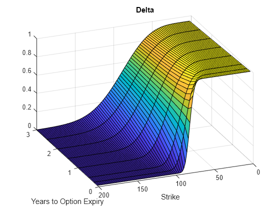
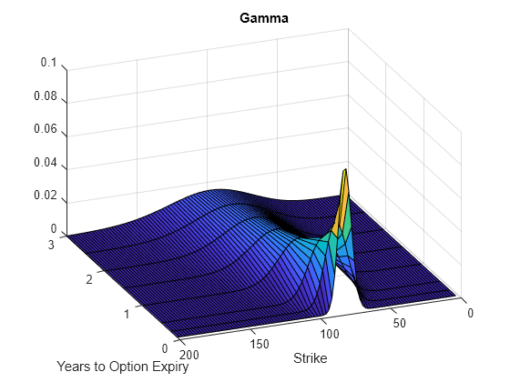
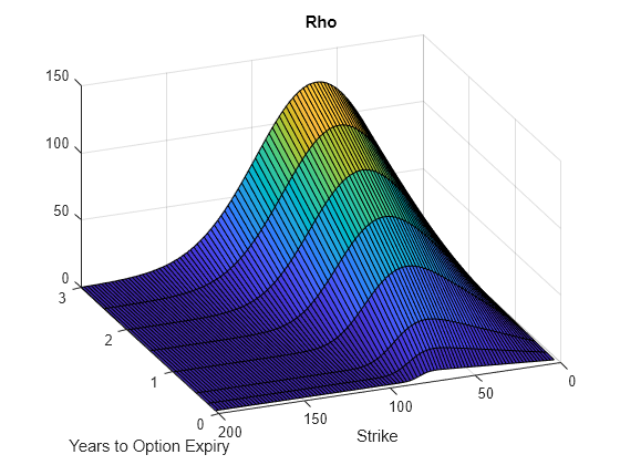
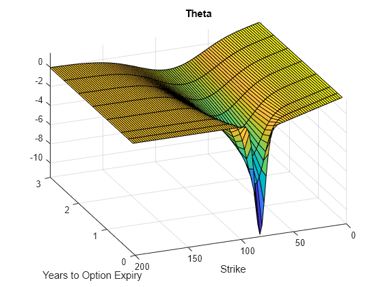
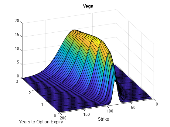
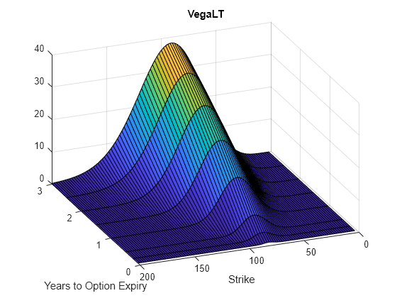
The Strike and Maturity inputs can be vectors. Set ExpandOutput to "true" to output the surfaces as NStrikes-by-NMaturities matrices.
Settle = datetime(2017,6,29);
Maturity = datemnth(Settle, 12*[1/12 0.25 (0.5:0.5:3)]');
Times = yearfrac(Settle, Maturity);
Strike = (2:2:200)';

[Delta, Gamma, Rho, Theta, Vega, VegaLT] = ...
    optSensByHestonNI(Rate, AssetPrice, Settle, Maturity, OptSpec, Strike, ...
    V0, ThetaV, Kappa, SigmaV, RhoSV, 'DividendYield', DividendYield, ...
    'OutSpec', ["delta", "gamma", "rho", "theta", "vega", "vegalt"], ...
    'ExpandOutput', true);

[X,Y] = meshgrid(Times,Strike);

figure;
surf(X,Y,Delta);
title('Delta');
xlabel('Years to Option Expiry');
ylabel('Strike');
view(-112,34);
xlim([0 Times(end)]);
figure;
surf(X,Y,Gamma)
title('Gamma')
xlabel('Years to Option Expiry')
ylabel('Strike')
view(-112,34);
xlim([0 Times(end)]);
figure;
surf(X,Y,Rho)
title('Rho')
xlabel('Years to Option Expiry')
ylabel('Strike')
view(-112,34);
xlim([0 Times(end)]);
figure;
surf(X,Y,Theta)
title('Theta')
xlabel('Years to Option Expiry')
ylabel('Strike')
view(-112,34);
xlim([0 Times(end)]);
figure;
surf(X,Y,Vega)
title('Vega')
xlabel('Years to Option Expiry')
ylabel('Strike')
view(-112,34);
xlim([0 Times(end)]);
figure;
surf(X,Y,VegaLT)
title('VegaLT')
xlabel('Years to Option Expiry')
ylabel('Strike')
view(-112,34);
xlim([0 Times(end)]);
Input Arguments
Rate — Continuously compounded risk-free interest rate
decimal
Continuously compounded risk-free interest rate, specified as a scalar decimal value.
Data Types: double
AssetPrice — Current underlying asset price
numeric
Current underlying asset price, specified as numeric value using a scalar or a
NINST-by-1 or
NColumns-by-1 vector.
For more information on the proper dimensions for AssetPrice,
see the name-value pair argument ExpandOutput.
Data Types: double
Settle — Option settlement date
datetime array | string array | date character vector
Option settlement date, specified as a
NINST-by-1 or
NColumns-by-1 vector using a datetime array,
string array, or date character vectors. The Settle date must be
before the Maturity date.
To support existing code, optSensByHestonNI also
accepts serial date numbers as inputs, but they are not recommended.
For more information on the proper dimensions for Settle, see
the name-value pair argument ExpandOutput.
Maturity — Option maturity date
datetime array | string array | date character vector
Option maturity date, specified as a
NINST-by-1 or
NColumns-by-1 vector using a datetime array,
string array, or date character vectors.
To support existing code, optSensByHestonNI also
accepts serial date numbers as inputs, but they are not recommended.
For more information on the proper dimensions for Maturity, see
the name-value pair argument ExpandOutput.
OptSpec — Definition of option
cell array of character vector with values 'call' or 'put' | string array with values "call" or "put"
Definition of the option, specified as a
NINST-by-1 or
NColumns-by-1 vector using a cell array of
character vectors or string arrays with values 'call' or
'put'.
For more information on the proper dimensions for OptSpec, see
the name-value pair argument ExpandOutput.
Data Types: cell | string
Strike — Option strike price value
numeric
Option strike price value, specified as a
NINST-by-1,
NRows-by-1,
NRows-by-NColumns vector of strike
prices.
For more information on the proper dimensions for Strike, see
the name-value pair argument ExpandOutput.
Data Types: double
V0 — Initial variance of underlying asset
numeric
Initial variance of the underling asset, specified as a scalar numeric value.
Data Types: double
ThetaV — Long-term variance of underlying asset
numeric
Long-term variance of the underling asset, specified as a scalar numeric value.
Data Types: double
Kappa — Mean revision speed for the variance of underlying asset
numeric
Mean revision speed for the underling asset, specified as a scalar numeric value.
Data Types: double
SigmaV — Volatility of the variance of underlying asset
numeric
Volatility of the variance of the underling asset, specified as a scalar numeric value.
Data Types: double
RhoSV — Correlation between Wiener processes for underlying asset and its variance
numeric
Correlation between the Wiener processes for the underlying asset and its variance, specified as a scalar numeric value.
Data Types: double
Name-Value Arguments
Specify optional pairs of arguments as
Name1=Value1,...,NameN=ValueN, where Name is
the argument name and Value is the corresponding value.
Name-value arguments must appear after other arguments, but the order of the
pairs does not matter.
Before R2021a, use commas to separate each name and value, and enclose
Name in quotes.
Example: PriceSens = optSensByHestonFFT(Rate, AssetPrice, Settle,Maturity,
OptSpec, Strike, V0, ThetaV, Kappa, SigmaV, RhoSV,'Basis',7)
Basis — Day-count basis of instrument
0 (default) | numeric values: 0,1, 2, 3, 4, 6, 7, 8,
9, 10, 11,
12, 13
Day-count of the instrument, specified as the comma-separated pair consisting of
'Basis' and a scalar using a supported value:
0 = actual/actual
1 = 30/360 (SIA)
2 = actual/360
3 = actual/365
4 = 30/360 (PSA)
5 = 30/360 (ISDA)
6 = 30/360 (European)
7 = actual/365 (Japanese)
8 = actual/actual (ICMA)
9 = actual/360 (ICMA)
10 = actual/365 (ICMA)
11 = 30/360E (ICMA)
12 = actual/365 (ISDA)
13 = BUS/252
For more information, see Basis.
Data Types: double
DividendYield — Continuously compounded underlying asset yield
0 (default) | numeric
Continuously compounded underlying asset yield, specified as the comma-separated
pair consisting of 'DividendYield' and a scalar numeric
value.
Data Types: double
VolRiskPremium — Volatility risk premium
0 (default) | numeric
Volatility risk premium, specified as the comma-separated pair consisting of
'VolRiskPremium' and a scalar numeric value.
Data Types: double
LittleTrap — Flag indicating Little Heston Trap formulation
true (default) | logical with values true or false
Flag indicating Little Heston Trap formulation by Albrecher
et
al, specified as the comma-separated pair consisting of
'LittleTrap' and a logical:
true— Use the Albrecher et al formulation.false— Use the original Heston formation.
Data Types: logical
OutSpec — Define outputs
["price"] (default) | string array with values "price", "delta", "gamma", "vega",
"rho", "theta", and
"vegalt" | cell array of character vectors with values 'price',
'delta', 'gamma', 'vega',
'rho', 'theta', and
'vegalt'
Define outputs, specified as the comma-separated pair consisting of
'OutSpec' and a NOUT-
by-1 or a 1-by-NOUT
string array or cell array of character vectors with supported values.
Note
"vega" is the sensitivity with respect the initial
volatility sqrt(V0). In contrast,
"vegalt" is the sensitivity with respect to the long-term
volatility sqrt(ThetaV).
Example: OutSpec =
["price","delta","gamma","vega","rho","theta","vegalt"]
Data Types: string | cell
AbsTol — Absolute error tolerance for numerical integration
1e-10 (default) | numeric
Absolute error tolerance for numerical integration, specified as the
comma-separated pair consisting of 'AbsTol' and a scalar numeric
value.
Data Types: double
RelTol — Relative error tolerance for numerical integration
1e-6 (default) | numeric
Relative error tolerance for numerical integration, specified as the
comma-separated pair consisting of 'RelTol' and a scalar numeric
value.
Data Types: double
IntegrationRange — Numerical integration range used to approximate continuous integral over [0 Inf]
[1e-9 Inf] (default) | vector
Numerical integration range used to approximate the continuous integral over
[0 Inf], specified as the comma-separated pair consisting of
'IntegrationRange' and a 1-by-2
vector representing [LowerLimit UpperLimit].
Data Types: double
Framework — Framework for computing option prices and sensitivities using numerical integration of models
"heston1993" (default) | string with values "heston1993" or
"lewis2001"
| character vector with values 'heston1993' or
'lewis2001'
Framework for computing option prices and sensitivities using numerical
integration of models, specified as the comma-separated pair consisting of
'Framework' and a scalar string or character vector with the
following values:
"heston1993"or'heston1993'— Method used in Heston (1993)"lewis2001"or'lewis2001'— Method used in Lewis (2001)
Data Types: char | string
ExpandOutput — Flag to expand the outputs
false (outputs are NINST-by-1 vectors) (default) | logical with value of true or false
Flag to expand the outputs, specified as the comma-separated pair consisting of
'ExpandOutput' and a logical:
true— Iftrue, the outputs areNRows-by-NColumnsmatrices.NRowsis the number of strikes for each column and it is determined by theStrikeinput. For example,Strikecan be aNRows-by-1vector, or aNRows-by-NColumnsmatrix.NColumnsis determined by the sizes ofAssetPrice,Settle,Maturity, andOptSpec, which must all be either scalar orNColumns-by-1vectors.false— Iffalse, the outputs areNINST-by-1vectors. Also, the inputsStrike,AssetPrice,Settle,Maturity, andOptSpecmust all be either scalar orNINST-by-1vectors.
Data Types: logical
Output Arguments
PriceSens — Option prices or sensitivities
numeric
Option prices or sensitivities, returned as a
NINST-by-1, or
NRows-by-NColumns, depending on
ExpandOutput. The name-value pair argument
OutSpec determines the types and order of the outputs.
More About
Vanilla Option
A vanilla option is a category of options that includes only the most standard components.
A vanilla option has an expiration date and straightforward strike price. American-style options and European-style options are both categorized as vanilla options.
The payoff for a vanilla option is as follows:
For a call:
For a put:
where:
St is the price of the underlying asset at time t.
K is the strike price.
For more information, see Vanilla Option.
Heston Stochastic Volatility Model
The Heston model is an extension of the Black-Scholes model, where the volatility (square root of variance) is no longer assumed to be constant, and the variance now follows a stochastic (CIR) process. This allows modeling the implied volatility smiles observed in the market.
The stochastic differential equation is:
where
r is the continuous risk-free rate.
q is the continuous dividend yield.
St is the asset price at time t.
vt is the asset price variance at time t.
v0 is the initial variance of the asset price at t = 0 for (v0 > 0).
θ is the long-term variance level for (θ > 0).
κ is the mean reversion speed for the variance for (κ > 0).
σv is the volatility of the variance for (σv > 0).
p is the correlation between the Wiener processes Wt and Wvt for (-1 ≤ p ≤ 1).
The characteristic function for j = 1 (asset price measure) and j = 2 (risk-neutral measure) is:
where
ϕ is the characteristic function variable.
ƛVolRisk is the volatility risk premium.
τ is the time to maturity (τ = T - t).
i is the unit imaginary number (i2 = -1).
The definitions for Cj and Dj under “The Little Heston Trap” by Albrecher et al. (2007) are:
Numerical Integration Method Under Heston (1993) Framework
Numerical integration is used to evaluate the continuous integral for the inverse Fourier transform.
The numerical integration method under the Heston (1993) framework is based on the following expressions:
where
r is the continuous risk-free rate.
q is the continuous dividend yield.
St is the asset price at time t.
K is the strike.
τ is time to maturity (τ = T-t).
Call(K) is the call price at strike K.
Put(K) is the put price at strike K.
i is a unit imaginary number (i2= -1).
ϕ is the characteristic function variable.
fj(ϕ) is the characteristic function for Pj(j = 1,2).
P1 is the probability of St > K under the asset price measure for the model.
P2 is the probability of St > K under the risk-neutral measure for the model.
Where j = 1,2 so that f1(ϕ) and f2(ϕ) are the characteristic functions for probabilities P1 and P2, respectively.
This framework is chosen with the default value “Heston1993” for the
Framework name-value pair argument.
Numerical Integration Method Under Lewis (2001) Framework
Numerical integration is used to evaluate the continuous integral for the inverse Fourier transform.
The numerical integration method under the Lewis (2001) framework is based on the following expressions:
where
r is the continuous risk-free rate.
q is the continuous dividend yield.
St is the asset price at time t.
K is the strike.
τ is time to maturity (τ = T-t).
Call(K) is the call price at strike K.
Put(K) is the put price at strike K.
i is a unit imaginary number (i2= -1).
ϕ is the characteristic function variable.
u is the characteristic function variable for integration, where .
f2(ϕ) is the characteristic function for P2.
P2 is the probability of St > K under the risk-neutral measure for the model.
This framework is chosen with the value “Lewis2001” for the
Framework name-value pair argument.
References
[1] Heston, S. L. “A Closed-Form Solution for Options with Stochastic Volatility with Applications to Bond and Currency Options.” The Review of Financial Studies. Vol 6. No. 2. 1993.
[2] Lewis, A. L. “A Simple Option Formula for General Jump-Diffusion and Other Exponential Levy Processes.” Envision Financial Systems and OptionCity.net, 2001.
Version History
Introduced in R2018aR2022b: Serial date numbers not recommended
Although optSensByHestonNI supports serial date numbers,
datetime values are recommended instead. The
datetime data type provides flexible date and time
formats, storage out to nanosecond precision, and properties to account for time
zones and daylight saving time.
To convert serial date numbers or text to datetime values, use the datetime function. For example:
t = datetime(738427.656845093,"ConvertFrom","datenum");
y = year(t)
y =

        2021
There are no plans to remove support for serial date number inputs.
MATLAB Command
You clicked a link that corresponds to this MATLAB command:
Run the command by entering it in the MATLAB Command Window. Web browsers do not support MATLAB commands.

Select a Web Site
Choose a web site to get translated content where available and see local events and offers. Based on your location, we recommend that you select: .
You can also select a web site from the following list
How to Get Best Site Performance
Select the China site (in Chinese or English) for best site performance. Other bat365 country sites are not optimized for visits from your location.
Americas
- América Latina (Español)
- Canada (English)
- United States (English)
Europe
- Belgium (English)
- Denmark (English)
- Deutschland (Deutsch)
- España (Español)
- Finland (English)
- France (Français)
- Ireland (English)
- Italia (Italiano)
- Luxembourg (English)
- Netherlands (English)
- Norway (English)
- Österreich (Deutsch)
- Portugal (English)
- Sweden (English)
- Switzerland
- United Kingdom (English)
Asia Pacific
- Australia (English)
- India (English)
- New Zealand (English)
- 中国
- 日本Japanese (日本語)
- 한국Korean (한국어)