Simulating Equity Prices
Simulating Multidimensional Market Models
This example compares alternative implementations of a separable multivariate
geometric Brownian motion process that is often referred to as a
multidimensional market model. It simulates sample paths of
an equity index portfolio using sde, sdeddo, sdeld, cev, and gbm objects.
The market model to simulate is:
| (1) |
where:
μ is a diagonal matrix of expected index returns.
D is a diagonal matrix with Xt along the diagonal.
σ is a diagonal matrix of standard deviations of index returns.
Representing Market Models Using SDE Objects
Create an sde object using sde to represent the equity
market model.
Load the
Data_GlobalIdx2data set:load Data_GlobalIdx2 prices = [Dataset.TSX Dataset.CAC Dataset.DAX ... Dataset.NIK Dataset.FTSE Dataset.SP];
Convert daily prices to returns:
returns = tick2ret(prices);
Compute data statistics to input to simulation methods:
nVariables = size(returns, 2); expReturn = mean(returns); sigma = std(returns); correlation = corrcoef(returns); t = 0; X = 100; X = X(ones(nVariables,1));
Create simple anonymous drift and diffusion functions accessible by (t, Xt):
F = @(t,X) diag(expReturn) * X; G = @(t,X) diag(X) * diag(sigma);
Use these functions with
sdeto create ansdeobject to represent the market model in Equation 1:SDE = sde(F, G, 'Correlation', correlation, 'StartState', X)
SDE = Class SDE: Stochastic Differential Equation ------------------------------------------- Dimensions: State = 6, Brownian = 6 ------------------------------------------- StartTime: 0 StartState: 100 (6x1 double array) Correlation: 6x6 double array Drift: drift rate function F(t,X(t)) Diffusion: diffusion rate function G(t,X(t)) Simulation: simulation method/function simByEulerThe
sdeobject requires additional information to determine the dimensionality of the model, because the functions passed to thesdeobject are known only by their (t, Xt) interface. In other words, thesdeobject requires only two inputs: a drift-rate function and a diffusion-rate function, both accessible by passing the sample time and the corresponding state vector (t, Xt).In this case, this information is insufficient to determine unambiguously the dimensionality of the state vector and Brownian motion. You resolve the dimensionality by specifying an initial state vector,
StartState. The SDE engine has assigned the default simulation method,simByEuler, to theSimulationparameter.
Representing Market Models Using SDEDDO Objects
Create an sdeddo object using sdeddo to represent the market
model in Equation 1:
Load the
Data_GlobalIdx2data set:load Data_GlobalIdx2 prices = [Dataset.TSX Dataset.CAC Dataset.DAX ... Dataset.NIK Dataset.FTSE Dataset.SP];
Convert daily prices to returns:
returns = tick2ret(prices);
Compute data statistics to input to simulation methods:
nVariables = size(returns, 2); expReturn = mean(returns); sigma = std(returns); correlation = corrcoef(returns);
Create
driftanddiffusionobjects usingdriftanddiffusion:F = drift(zeros(nVariables,1), diag(expReturn))
F = Class DRIFT: Drift Rate Specification ------------------------------------- Rate: drift rate function F(t,X(t)) A: 6x1 double array B: 6x6 diagonal double arrayG = diffusion(ones(nVariables,1), diag(sigma))
G = Class DIFFUSION: Diffusion Rate Specification --------------------------------------------- Rate: diffusion rate function G(t,X(t)) Alpha: 6x1 double array Sigma: 6x6 diagonal double arrayPass the
driftanddiffusionobjects tosdeddo:SDEDDO = sdeddo(F, G, 'Correlation', correlation, ... 'StartState', 100)
SDEDDO = Class SDEDDO: SDE from Drift and Diffusion Objects -------------------------------------------------- Dimensions: State = 6, Brownian = 6 -------------------------------------------------- StartTime: 0 StartState: 100 (6x1 double array) Correlation: 6x6 double array Drift: drift rate function F(t,X(t)) Diffusion: diffusion rate function G(t,X(t)) Simulation: simulation method/function simByEuler A: 6x1 double array B: 6x6 diagonal double array Alpha: 6x1 double array Sigma: 6x6 diagonal double arrayThe
sdeddoobject requires two input objects that provide more information than the two functions from step 4 of Representing Market Models Using SDE Objects. Thus, the dimensionality is more easily resolved. In fact, the initial price of each index is as a scalar (StartState=100). This is in contrast to thesdeobject, which required an explicit state vector to uniquely determine the dimensionality of the problem.Once again, the class of each object is clearly identified, and parameters display like fields of a structure. In particular, the
Rateparameter of drift and diffusion objects is identified as a callable function of time and state, F(t,Xt) and G(t,Xt), respectively. The additional parameters,A,B,Alpha, andSigma, are arrays of appropriate dimension, indicating static (non-time-varying) parameters. In other words, A(t,Xt), B(t,Xt), Alpha(t,Xt), and Sigma(t,Xt) are constant functions of time and state.
Representing Market Models Using SDELD, CEV, and GBM Objects
Create sdeld, cev, and gbm objects to represent the market
model in Equation 1.
Load the
Data_GlobalIdx2data set:load Data_GlobalIdx2 prices = [Dataset.TSX Dataset.CAC Dataset.DAX ... Dataset.NIK Dataset.FTSE Dataset.SP];
Convert daily prices to returns:
returns = tick2ret(prices);
Compute data statistics to input to simulation methods:
nVariables = size(returns, 2); expReturn = mean(returns); sigma = std(returns); correlation = corrcoef(returns); t = 0; X = 100; X = X(ones(nVariables,1));
Create an
sdeldobject usingsdeld:SDELD = sdeld(zeros(nVariables,1), diag(expReturn), ... ones(nVariables,1), diag(sigma),'Correlation', ... correlation, 'StartState', X)
SDELD = Class SDELD: SDE with Linear Drift ---------------------------------------- Dimensions: State = 6, Brownian = 6 ---------------------------------------- StartTime: 0 StartState: 100 (6x1 double array) Correlation: 6x6 double array Drift: drift rate function F(t,X(t)) Diffusion: diffusion rate function G(t,X(t)) Simulation: simulation method/function simByEuler A: 6x1 double array B: 6x6 diagonal double array Alpha: 6x1 double array Sigma: 6x6 diagonal double arrayCreate a
cevobject usingcev:CEV = cev(diag(expReturn), ones(nVariables,1), ... diag(sigma), 'Correlation', correlation, ... 'StartState', X)
CEV = Class CEV: Constant Elasticity of Variance ------------------------------------------ Dimensions: State = 6, Brownian = 6 ------------------------------------------ StartTime: 0 StartState: 100 (6x1 double array) Correlation: 6x6 double array Drift: drift rate function F(t,X(t)) Diffusion: diffusion rate function G(t,X(t)) Simulation: simulation method/function simByEuler Return: 6x6 diagonal double array Alpha: 6x1 double array Sigma: 6x6 diagonal double arrayCreate a
gbmobject usinggbm:GBM = gbm(diag(expReturn), diag(sigma), 'Correlation', ... correlation, 'StartState', X)
GBM = Class GBM: Generalized Geometric Brownian Motion ------------------------------------------------ Dimensions: State = 6, Brownian = 6 ------------------------------------------------ StartTime: 0 StartState: 100 (6x1 double array) Correlation: 6x6 double array Drift: drift rate function F(t,X(t)) Diffusion: diffusion rate function G(t,X(t)) Simulation: simulation method/function simByEuler Return: 6x6 diagonal double array Sigma: 6x6 diagonal double arrayNote the succession of interface restrictions:
However, all three objects represent the same multidimensional market model.
Also,
cevandgbmobjects display the underlying parameterBderived from thesdeldobject asReturn. This is an intuitive name commonly associated with equity models.
Simulating Equity Markets Using the Default Simulate Method
Load the
Data_GlobalIdx2data set and usesdeto specify the SDE model as in Representing Market Models Using SDE Objects.load Data_GlobalIdx2 prices = [Dataset.TSX Dataset.CAC Dataset.DAX ... Dataset.NIK Dataset.FTSE Dataset.SP]; returns = tick2ret(prices); nVariables = size(returns,2); expReturn = mean(returns); sigma = std(returns); correlation = corrcoef(returns); t = 0; X = 100; X = X(ones(nVariables,1)); F = @(t,X) diag(expReturn)* X; G = @(t,X) diag(X) * diag(sigma); SDE = sde(F, G, 'Correlation', ... correlation, 'StartState', X);
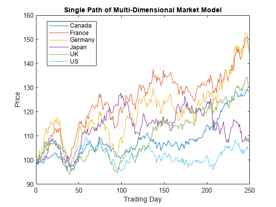
Simulate a single path of correlated equity index prices over one calendar year (defined as approximately 250 trading days) using the default
simulatemethod:nPeriods = 249; % # of simulated observations dt = 1; % time increment = 1 day rng(142857,'twister') [S,T] = simulate(SDE, nPeriods, 'DeltaTime', dt); whos S
Name Size Bytes Class Attributes S 250x6 12000 double
The output array
Sis a 250-by-6 = (NPeriods + 1-by-nVariables-by-1) array with the same initial value,100, for all indices. Each row ofSis an observation of the state vector Xt at time t.Plot the simulated paths.
plot(T, S), xlabel('Trading Day'), ylabel('Price') title('Single Path of Multi-Dimensional Market Model') legend({'Canada' 'France' 'Germany' 'Japan' 'UK' 'US'}, ... 'Location', 'Best')
Simulating Equity Markets Using the SimByEuler Method
Because simByEuler is a valid
simulation method, you can call it directly, overriding the
Simulation parameter's current method or function (which
in this case is simByEuler). The following statements
produce the same price paths as generated in Simulating Equity Markets Using the Default Simulate Method:
Load the
Data_GlobalIdx2data set and usesdeto specify the SDE model as in Representing Market Models Using SDE Objects.load Data_GlobalIdx2 prices = [Dataset.TSX Dataset.CAC Dataset.DAX ... Dataset.NIK Dataset.FTSE Dataset.SP]; returns = tick2ret(prices); nVariables = size(returns,2); expReturn = mean(returns); sigma = std(returns); correlation = corrcoef(returns); t = 0; X = 100; X = X(ones(nVariables,1)); F = @(t,X) diag(expReturn)* X; G = @(t,X) diag(X) * diag(sigma); SDE = sde(F, G, 'Correlation', ... correlation, 'StartState', X);
Simulate a single path using
simByEuler.nPeriods = 249; % # of simulated observations dt = 1; % time increment = 1 day rng(142857,'twister') [S,T] = simByEuler(SDE, nPeriods, 'DeltaTime', dt);
Simulate 10 trials with the same initial conditions, and examine
S:rng(142857,'twister') [S,T] = simulate(SDE, nPeriods, 'DeltaTime', dt, 'nTrials', 10); whos S
Name Size Bytes Class Attributes S 250x6x10 120000 double
Now the output array
Sis anNPeriods + 1-by-nVariables-by-NTrialstime series array.Plot the first paths.
plot(T, S(:,:,1)), xlabel('Trading Day'), ylabel('Price') title('First Path of Multi-Dimensional Market Model') legend({'Canada' 'France' 'Germany' 'Japan' 'UK' 'US'},... 'Location', 'Best')

The first realization of S is identical to the paths in the
plot.
Simulating Equity Markets Using GBM Simulation Methods
Finally, consider simulation using GBM simulation methods.
Separable GBM models have two specific simulation
methods:
An overloaded Euler simulation method,
simByEuler, designed for optimal performanceA function,
simBySolution, provides an approximate solution of the underlying stochastic differential equation, designed for accuracy
Load the
Data_GlobalIdx2data set and usesdeto specify the SDE model as in Representing Market Models Using SDE Objects, and the GBM model as in Representing Market Models Using SDELD, CEV, and GBM Objects.load Data_GlobalIdx2 prices = [Dataset.TSX Dataset.CAC Dataset.DAX ... Dataset.NIK Dataset.FTSE Dataset.SP]; returns = tick2ret(prices); nVariables = size(returns,2); expReturn = mean(returns); sigma = std(returns); correlation = corrcoef(returns); t = 0; X = 100; X = X(ones(nVariables,1)); F = @(t,X) diag(expReturn)* X; G = @(t,X) diag(X) * diag(sigma); SDE = sde(F, G, 'Correlation', ... correlation, 'StartState', X); GBM = gbm(diag(expReturn),diag(sigma), 'Correlation', ... correlation, 'StartState', X);
To illustrate the performance benefit of the overloaded Euler approximation method, increase the number of trials to
10000.nPeriods = 249; % # of simulated observations dt = 1; % time increment = 1 day rng(142857,'twister') [X,T] = simulate(GBM, nPeriods, 'DeltaTime', dt, ... 'nTrials', 10000); whos X
Name Size Bytes Class Attributes X 250x6x10000 120000000 double
The output
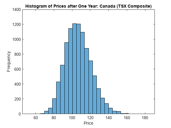
Xis a much larger time series array.Using this sample size, examine the terminal distribution of Canada's TSX Composite to verify qualitatively the lognormal character of the data.
histogram(squeeze(X(end,1,:)), 30), xlabel('Price'), ylabel('Frequency') title('Histogram of Prices after One Year: Canada (TSX Composite)')
Simulate 10 trials of the solution and plot the first trial:
rng(142857,'twister') [S,T] = simulate(SDE, nPeriods, 'DeltaTime', dt, 'nTrials', 10); rng(142857,'twister') [X,T] = simBySolution(GBM, nPeriods,... 'DeltaTime', dt, 'nTrials', 10); subplot(2,1,1) plot(T, S(:,:,1)), xlabel('Trading Day'),ylabel('Price') title('1st Path of Multi-Dim Market Model:Euler Approximation') subplot(2,1,2) plot(T, X(:,:,1)), xlabel('Trading Day'),ylabel('Price') title('1st Path of Multi-Dim Market Model:Analytic Solution')
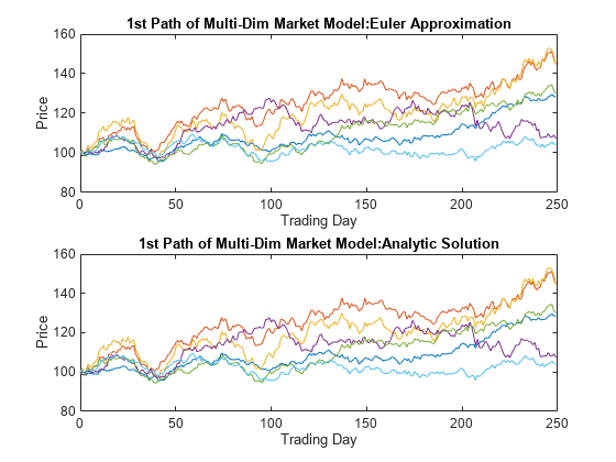
In this example, all parameters are constants, and
simBySolutiondoes indeed sample the exact solution. The details of a single index for any given trial show that the price paths of the Euler approximation and the exact solution are close, but not identical.The following plot illustrates the difference between the two methods:
subplot(1,1,1) plot(T, S(:,1,1) - X(:,1,1), 'blue'), grid('on') xlabel('Trading Day'), ylabel('Price Difference') title('Euler Approx Minus Exact Solution:Canada(TSX Composite)')
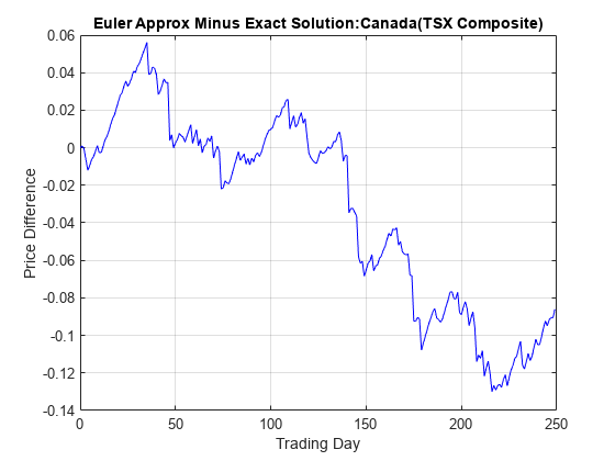
The simByEuler Euler
approximation literally evaluates the stochastic differential equation directly
from the equation of motion, for some suitable value of the
dt time increment. This simple approximation suffers from
discretization error. This error is attributed to the discrepancy between the
choice of the dt time increment and what in theory is a
continuous-time parameter.
The discrete-time approximation improves as DeltaTime
approaches zero. The Euler method is often the least accurate and most general
method available. All models shipped in the simulation suite have this
method.
In contrast, thesimBySolution method provides
a more accurate description of the underlying model. This method simulates the
price paths by an approximation of the closed-form solution of separable models.
Specifically, it applies a Euler approach to a transformed process, which in
general is not the exact solution to this GBM model. This is
because the probability distributions of the simulated and true state vectors
are identical only for piecewise constant parameters.
When all model parameters are piecewise constant over each observation period,
the simulated process is exact for the observation times at which the state
vector is sampled. Since all parameters are constants in this example,simBySolution does indeed
sample the exact solution.
For an example of how to use simBySolution to optimize the
accuracy of solutions, see Optimizing Accuracy: About Solution Precision and Error.
Inducing Dependence and Correlation
This example illustrates two techniques that induce dependence between individual
elements of a state vector. It also illustrates the interaction between
Sigma and Correlation.
The first technique generates correlated Gaussian variates to form a Brownian
motion process with dependent components. These components are then weighted by a
diagonal volatility or exposure matrix Sigma.
The second technique generates independent Gaussian variates to form a standard
Brownian motion process, which is then weighted by the lower Cholesky factor of the
desired covariance matrix. Although these techniques can be used on many models, the
relationship between them is most easily illustrated by working with a separable
GBM model (see Simulating Equity Prices Using
GBM Simulation Methods). The market model to simulate is:
where μ is a diagonal matrix.
Load the data set:
load Data_GlobalIdx2
prices  = [Dataset.TSX Dataset.CAC Dataset.DAX ...
Dataset.NIK Dataset.FTSE Dataset.SP];
Convert the daily prices to returns:
returns = tick2ret(prices);
Specify
SigmaandCorrelationusing the first technique:Using the first technique, specify
Sigmaas a diagonal matrix of asset return standard deviations:expReturn = diag(mean(returns)); % expected return vector sigma = diag(std(returns)); % volatility of returns
Specify
Correlationas the sample correlation matrix of those returns. In this case, the components of the Brownian motion are dependent:correlation = corrcoef(returns); GBM1 = gbm(expReturn,sigma,'Correlation',... correlation);
Specify
SigmaandCorrelationusing the second technique:Using the second technique, specify
Sigmaas the lower Cholesky factor of the asset return covariance matrix:covariance = cov(returns); sigma = cholcov(covariance)';
Set
Correlationto an identity matrix:GBM2 = gbm(expReturn,sigma);
Here,
sigmacaptures both the correlation and magnitude of the asset return uncertainty. In contrast to the first technique, the components of the Brownian motion are independent. Also, this technique accepts the default assignment of an identity matrix toCorrelation, and is more straightforward.
Simulate a single trial of 1000 observations (roughly four years of daily data) using both techniques. By default, all state variables start at
1:rng(22814,'twister') [X1,T] = simByEuler(GBM1,1000); % correlated Brownian motion rng(22814,'twister') [X2,T] = simByEuler(GBM2,1000); % standard Brownian motion
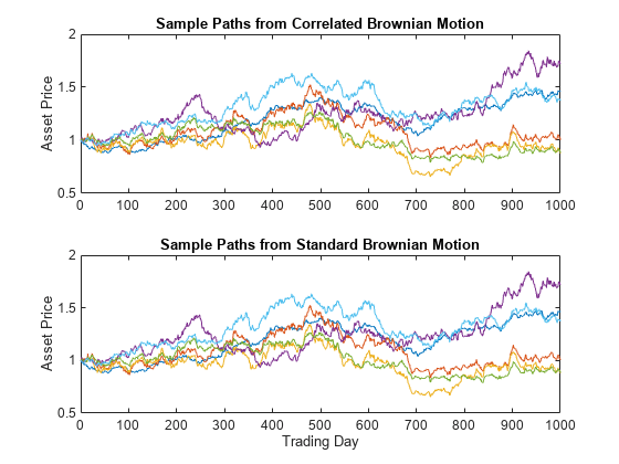
When based on the same initial random number state, each technique generates identical asset price paths:
subplot(2,1,1)
plot(T, X1)
title('Sample Paths from Correlated Brownian Motion')
ylabel('Asset Price')
subplot(2,1,2)
plot(T, X2)
title('Sample Paths from Standard Brownian Motion')
xlabel('Trading Day')
ylabel('Asset Price')
Dynamic Behavior of Market Parameters
As discussed in Creating SDE Objects, object parameters may be evaluated as if they are MATLAB® functions accessible by a common interface. This accessibility provides the impression of dynamic behavior regardless of whether the underlying parameters are truly time-varying. Furthermore, because parameters are accessible by a common interface, seemingly simple linear constructs may in fact represent complex, nonlinear designs.
For example, consider a univariate geometric Brownian motion (GBM) model of the form:
In this model, the return, μ(t), and volatility,
σ(t), are dynamic parameters of time alone. However, when creating a
gbm object to represent the underlying
model, such dynamic behavior must be accessible by the common (t,
Xt) interface. This reflects the
fact that GBM models (and others) are restricted
parameterizations that derive from the general SDE class.
As a convenience, you can specify parameters of restricted models, such as
GBM models, as traditional MATLAB arrays of appropriate dimension. In this case, such arrays represent a
static special case of the more general dynamic situation accessible by the
(t, Xt)
interface.
Moreover, when you enter parameters as functions, object constructors can verify that they return arrays of correct size by evaluating them at the initial time and state. Otherwise, object constructors have no knowledge of any particular functional form.
The following example illustrates a technique that includes dynamic behavior by mapping a traditional MATLAB time series array to a callable function with a (t, Xt) interface. It also compares the function with an otherwise identical model with constant parameters.
Because time series arrays represent dynamic behavior that must be captured by
functions accessible by the (t,
Xt) interface, you need utilities
to convert traditional time series arrays into callable functions of time and state.
The following example shows how to do this using the conversion function ts2func (time series to
function).
Load the data. Load a daily historical data set containing three-month Euribor rates and closing index levels of France's CAC 40 spanning the time interval February 7, 2001 to April 24, 2006:
load Data_GlobalIdx2Simulate risk-neutral sample paths. Simulate risk-neutral sample paths of the CAC 40 index using a geometric Brownian motion (
GBM) model:where r(t) represents evolution of the risk-free rate of return.
Furthermore, assume that you need to annualize the relevant information derived from the daily data (annualizing the data is optional, but is useful for comparison to other examples), and that each calendar year comprises 250 trading days:
dt      = 1/250;
returns = tick2ret(Dataset.CAC);
sigma   = std(returns)*sqrt(250);
yields  = Dataset.EB3M;
yields  = 360*log(1 + yields);
Compare the sample paths from two risk-neutral historical simulation approaches. Compare the resulting sample paths obtained from two risk-neutral historical simulation approaches, where the daily Euribor yields serve as a proxy for the risk-free rate of return.
The first approach specifies the risk-neutral return as the sample average of Euribor yields, and therefore assumes a constant (non-dynamic) risk-free return:
nPeriods = length(yields);  % Simulated observations
rng(5713,'twister')
obj    = gbm(mean(yields),diag(sigma),'StartState',100)
obj =
   Class GBM: Generalized Geometric Brownian Motion
   ------------------------------------------------
     Dimensions: State = 1, Brownian = 1
   ------------------------------------------------
      StartTime: 0
     StartState: 100
    Correlation: 1
          Drift: drift rate function F(t,X(t))
      Diffusion: diffusion rate function G(t,X(t))
     Simulation: simulation method/function simByEuler
         Return: 0.0278117
          Sigma: 0.231906
[X1,T] = simulate(obj,nPeriods,'DeltaTime',dt);In contrast, the second approach specifies the risk-neutral return as the historical time series of Euribor yields. It therefore assumes a dynamic, yet deterministic, rate of return; this example does not illustrate stochastic interest rates. To illustrate this dynamic effect, use the
ts2funcutility:r = ts2func(yields,'Times',(0:nPeriods - 1)');ts2funcpackages a specified time series array inside a callable function of time and state, and synchronizes it with an optional time vector. For instance:r(0,100)
ans = 0.0470
evaluates the function at (t = 0, X t = 100) and returns the first observed Euribor yield. However, you can also evaluate the resulting function at any intermediate time t and state Xt:
r(7.5,200)
ans = 0.0472
Furthermore, the following command produces the same result when called with time alone:
r(7.5)
ans = 0.0472
The equivalence of these last two commands highlights some important features.
When you specify parameters as functions, they must evaluate properly when passed a scalar, real-valued sample time (t), and an NVars-by-
1state vector (Xt). They must also generate an array of appropriate dimensions, which in the first case is a scalar constant, and in the second case is a scalar, piecewise constant function of time alone.You are not required to use either time (t) or state (Xt). In the current example, the function evaluates properly when passed time followed by state, thereby satisfying the minimal requirements. The fact that it also evaluates correctly when passed only time simply indicates that the function does not require the state vector Xt. The important point to make is that it works when you pass it (t, Xt).
Furthermore, the
ts2funcfunction performs a zero-order-hold (ZOH) piecewise constant interpolation. The notion of piecewise constant parameters is pervasive throughout the SDE architecture, and is discussed in more detail in Optimizing Accuracy: About Solution Precision and Error.
Perform a second simulation using the same initial random number state. Complete the comparison by performing the second simulation using the same initial random number state:
rng(5713,'twister')
obj = gbm(r, diag(sigma),'StartState',100)
obj =
   Class GBM: Generalized Geometric Brownian Motion
   ------------------------------------------------
     Dimensions: State = 1, Brownian = 1
   ------------------------------------------------
      StartTime: 0
     StartState: 100
    Correlation: 1
          Drift: drift rate function F(t,X(t))
      Diffusion: diffusion rate function G(t,X(t))
     Simulation: simulation method/function simByEuler
         Return: function ts2func/vector2Function
          Sigma: 0.231906
X2 = simulate(obj,nPeriods,'DeltaTime',dt);Compare the two simulation trials. Plot the series of risk-free reference rates to compare the two simulation trials:
subplot(2,1,1)
plot(dates,100*yields)
datetick('x')
xlabel('Date')
ylabel('Annualized Yield (%)')
title('Risk Free Rate(3-Mo Euribor Continuously-Compounded)')
subplot(2,1,2)
plot(T,X1,'red',T,X2,'blue')
xlabel('Time (Years)')
ylabel('Index Level')
title('Constant vs. Dynamic Rate of Return: CAC 40')
legend({'Constant Interest Rates' 'Dynamic Interest Rates'},...
    'Location', 'Best')
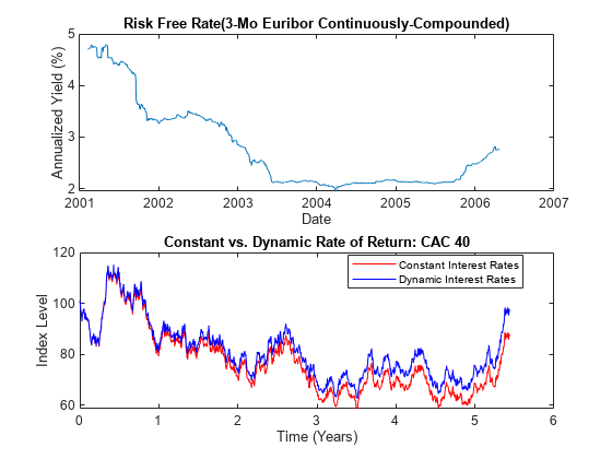
The paths are close but not exact. The blue line in the last plot uses all the historical Euribor data, and illustrates a single trial of a historical simulation.
Pricing Equity Options
As discussed in Ensuring Positive Interest Rates, all simulation and interpolation methods allow you to specify one or more functions of the form:
to evaluate at the end of every sample time.
The related example illustrates a simple, common end-of-period processing function to ensure nonnegative interest rates. This example illustrates a processing function that allows you to avoid simulation outputs altogether.
Consider pricing European stock options by Monte Carlo simulation within a Black-Scholes-Merton framework. Assume that the stock has the following characteristics:
The stock currently trades at 100.
The stock pays no dividends.
The stock's volatility is 50% per annum.
The option strike price is 95.
The option expires in three months.
The risk-free rate is constant at 10% per annum.
To solve this problem, model the evolution of the underlying stock by a univariate geometric Brownian motion (GBM) model with constant parameters:
Furthermore, assume that the stock price is simulated daily, and that each calendar month comprises 21 trading days:
The goal is to simulate independent paths of daily stock prices, and calculate the price of European options as the risk-neutral sample average of the discounted terminal option payoff at expiration 63 days from now. This example calculates option prices by two approaches:
A Monte Carlo simulation that explicitly requests the simulated stock paths as an output. The output paths are then used to price the options.
An end-of-period processing function, accessible by time and state, that records the terminal stock price of each sample path. This processing function is implemented as a nested function with access to shared information. For more information, see
Example_BlackScholes.m.
Before simulation, invoke the example file to access the end-of-period processing function:
nTrials = 10000; % Number of independent trials (i.e., paths)
f = Example_BlackScholes(nPeriods,nTrials)
f = struct with fields: BlackScholes: @Example_BlackScholes/saveTerminalStockPrice CallPrice: @Example_BlackScholes/getCallPrice PutPrice: @Example_BlackScholes/getPutPriceSimulate 10000 independent trials (sample paths). Request the simulated stock price paths as an output, and specify an end-of-period processing function:
rng(88161,'twister')
X = simBySolution(obj,nPeriods,'DeltaTime',dt,...
    'nTrials',nTrials,'Processes',f.BlackScholes);
Calculate the option prices directly from the simulated stock price paths. Because these are European options, ignore all intermediate stock prices:
call = mean(exp(-rate*T)*max(squeeze(X(end,:,:)) - strike, 0))
call = 13.9342
put = mean(exp(-rate*T)*max(strike - squeeze(X(end,:,:)), 0))
put = 6.4166
Price the options indirectly by invoking the nested functions:
f.CallPrice(strike,rate)
ans = 13.9342
f.PutPrice(strike,rate)
ans = 6.4166
For reference, the theoretical call and put prices computed from the Black-Scholes option formulas are
13.6953and6.3497, respectively.Although steps 3 and 4 produce the same option prices, the latter approach works directly with the terminal stock prices of each sample path. Therefore, it is much more memory efficient. In this example, there is no compelling reason to request an output.
See Also
sde | bm | gbm | merton | bates | drift | diffusion | sdeddo | sdeld | cev | cir | heston | hwv | sdemrd | ts2func | simulate | simByEuler | simBySolution | simByQuadExp | simBySolution | interpolate
Related Examples
- Simulating Interest Rates
- Stratified Sampling
- Price American Basket Options Using Standard Monte Carlo and Quasi-Monte Carlo Simulation
- Improving Performance of Monte Carlo Simulation with Parallel Computing
- Base SDE Models
- Drift and Diffusion Models
- Linear Drift Models
- Parametric Models
