Examine the Daily Closings of the Global Equity Index Data

The raw data consists of 2665 observations of daily closing values of the following representative equity indices spanning the trading dates 27-April-1993 to 14-July-2003:

  Canada: TSX Composite (Ticker ^GSPTSE)
  France: CAC 40        (Ticker ^FCHI)
 Germany: DAX           (Ticker ^GDAXI)
   Japan: Nikkei 225    (Ticker ^N225)
      UK: FTSE 100      (Ticker ^FTSE)
      US: S&P 500       (Ticker ^GSPC)

load Data_GlobalIdx1   % Import daily index closings

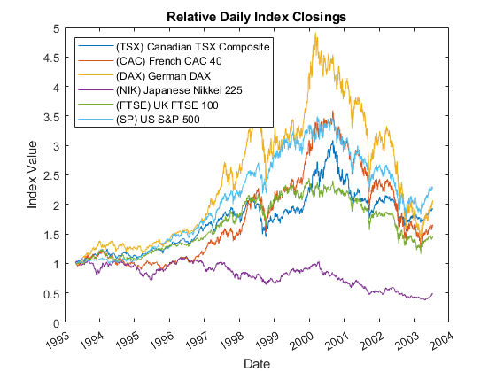
The following plot illustrates the relative price movements of each index. The initial level of each index has been normalized to unity to facilitate the comparison of relative performance, and no dividend adjustments are explicitly taken into account.

figure
plot(dates, ret2price(price2ret(Data)))
datetick('x')
xlabel('Date')
ylabel('Index Value')
title ('Relative Daily Index Closings')
legend(series, 'Location', 'NorthWest')

In preparation for subsequent modeling, convert the closing level of each index to daily logarithmic returns (sometimes called geometric, or continuously compounded, returns).

returns = price2ret(Data);    % Logarithmic returns
T       = size(returns,1);    % # of returns (i.e., historical sample size)

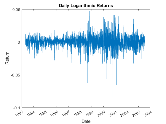
Since the first step in the overall modeling approach involves a repeated application of GARCH filtration and Extreme Value Theory to characterize the distribution of each individual equity index return series, it is helpful to examine the details for a particular country. You can change the next line of code to any integer in the set {1,2,3,4,5,6} to examine the details for any index.

index = 1;  % 1 = Canada, 2 = France, 3 = Germany, 4 = Japan, 5 = UK, 6 = US

figure
plot(dates(2:end), returns(:,index))
datetick('x')
xlabel('Date')
ylabel('Return')
title('Daily Logarithmic Returns')

Filter the Returns for Each Index

Modeling the tails of a distribution with a GPD requires the observations to be approximately independent and identically distributed (i.i.d.). However, most financial return series exhibit some degree of autocorrelation and, more importantly, heteroskedasticity.

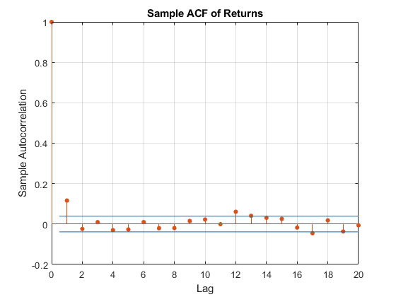
For example, the sample autocorrelation function (ACF) of the returns associated with the selected index reveal some mild serial correlation.

figure
autocorr(returns(:,index))
title('Sample ACF of Returns')

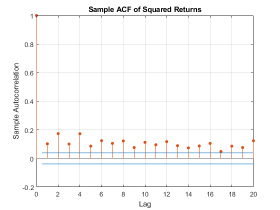
However, the sample ACF of the squared returns illustrates the degree of persistence in variance, and implies that GARCH modeling may significantly condition the data used in the subsequent tail estimation process.

figure
autocorr(returns(:,index).^2)
title('Sample ACF of Squared Returns')

To produce a series of i.i.d. observations, fit a first order autoregressive model to the conditional mean of the returns of each equity index

and an asymmetric GARCH model to the conditional variance

The first order autoregressive model compensates for autocorrelation, while the GARCH model compensates for heteroskedasticity. In particular, the last term incorporates asymmetry (leverage) into the variance by a Boolean indicator that takes the value 1 if the prior model residual is negative and 0 otherwise (see [3]).

Additionally, the standardized residuals of each index are modeled as a standardized Student's t distribution to compensate for the fat tails often associated with equity returns. That is

i.i.d. distributed

The following code segment extracts the filtered residuals and conditional variances from the returns of each equity index.

model     = arima('AR', NaN, 'Distribution', 't', 'Variance', gjr(1,1));
nIndices  = size(Data,2);        % # of indices
residuals = NaN(T, nIndices);    % preallocate storage
variances = NaN(T, nIndices);
fit       = cell(nIndices,1);

options   = optimoptions(@fmincon, 'Display', 'off', ...
    'Diagnostics', 'off', 'Algorithm', 'sqp', 'TolCon', 1e-7);

for i = 1:nIndices
    fit{i} = estimate(model, returns(:,i), 'Display', 'off', 'Options', options);
    [residuals(:,i), variances(:,i)] = infer(fit{i}, returns(:,i));
end

For the selected index, compare the model residuals and the corresponding conditional standard deviations filtered from the raw returns. The lower graph clearly illustrates the variation in volatility (heteroskedasticity) present in the filtered residuals.

figure
subplot(2,1,1)
plot(dates(2:end), residuals(:,index))
datetick('x')
xlabel('Date')
ylabel('Residual')
title ('Filtered Residuals')

subplot(2,1,2)
plot(dates(2:end), sqrt(variances(:,index)))
datetick('x')
xlabel('Date')
ylabel('Volatility')
title ('Filtered Conditional Standard Deviations')

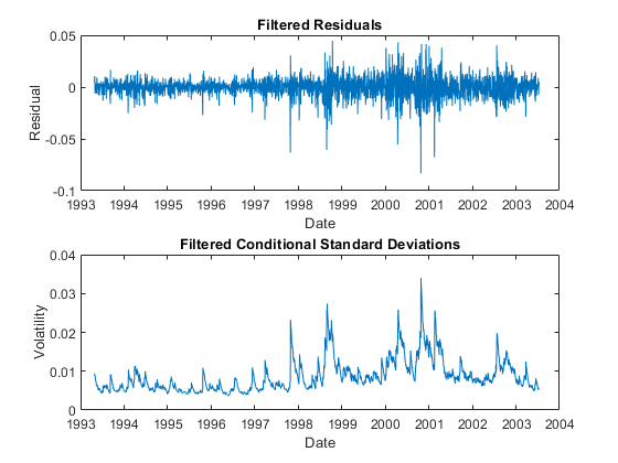
Having filtered the model residuals from each return series, standardize the residuals by the corresponding conditional standard deviation. These standardized residuals represent the underlying zero-mean, unit-variance, i.i.d. series upon which the EVT estimation of the sample CDF tails is based.

residuals = residuals ./ sqrt(variances);

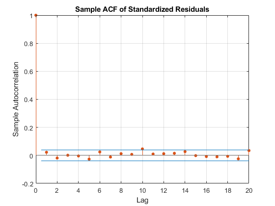
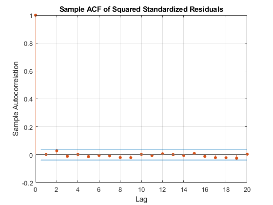
To conclude this section, examine the ACFs of the standardized residuals and squared standardized residuals.

Comparing the ACFs of the standardized residuals to the corresponding ACFs of the raw returns reveals that the standardized residuals are now approximately i.i.d., thereby far more amenable to subsequent tail estimation.

figure
autocorr(residuals(:,index))
title('Sample ACF of Standardized Residuals')

figure
autocorr(residuals(:,index).^2)
title('Sample ACF of Squared Standardized Residuals')

Estimate the Semi-Parametric CDFs

Given the standardized, i.i.d. residuals from the previous step, estimate the empirical CDF of each index with a Gaussian kernel. This smooths the CDF estimates, eliminating the staircase pattern of unsmoothed sample CDFs. Although non-parametric kernel CDF estimates are well suited for the interior of the distribution where most of the data is found, they tend to perform poorly when applied to the upper and lower tails. To better estimate the tails of the distribution, apply EVT to those residuals that fall in each tail.

Specifically, find upper and lower thresholds such that 10% of the residuals is reserved for each tail. Then fit the amount by which those extreme residuals in each tail fall beyond the associated threshold to a parametric GPD by maximum likelihood. This approach is often referred to as the distribution of exceedances or peaks over threshold method.

Given the exceedances in each tail, optimize the negative log-likelihood function to estimate the tail index (zeta) and scale (beta) parameters of the GPD.

The following code segment creates objects of type paretotails, one such object for each index return series. These paretotails objects encapsulate the estimates of the parametric GP lower tail, the non-parametric kernel-smoothed interior, and the parametric GP upper tail to construct a composite semi-parametric CDF for each index.

The resulting piecewise distribution object allows interpolation within the interior of the CDF and extrapolation (function evaluation) in each tail. Extrapolation is very desirable, allowing estimation of quantiles outside the historical record, and is invaluable for risk management applications.

Moreover, Pareto tail objects also provide methods to evaluate the CDF and inverse CDF (quantile function), and to query the cumulative probabilities and quantiles of the boundaries between each segment of the piecewise distribution.

nPoints      = 200;      % # of sampled points in each region of the CDF
tailFraction = 0.1;      % Decimal fraction of residuals allocated to each tail

tails = cell(nIndices,1);  % Cell array of Pareto tail objects

for i = 1:nIndices
    tails{i} = paretotails(residuals(:,i), tailFraction, 1 - tailFraction, 'kernel');
end

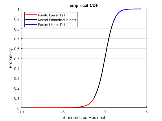
Having estimated the three distinct regions of the composite semi-parametric empirical CDF, graphically concatenate and display the result. Again, note that the lower and upper tail regions, displayed in red and blue, respectively, are suitable for extrapolation, while the kernel-smoothed interior, in black, is suitable for interpolation.

The code below calls the CDF and inverse CDF methods of the Pareto tails object of interest with data other than that upon which the fit is based. Specifically, the referenced methods have access to the fitted state, and are now invoked to select and analyze specific regions of the probability curve, acting as a powerful data filtering mechanism.

figure
hold on
grid on

minProbability = cdf(tails{index}, (min(residuals(:,index))));
maxProbability = cdf(tails{index}, (max(residuals(:,index))));

pLowerTail = linspace(minProbability  , tailFraction    , nPoints); % sample lower tail
pUpperTail = linspace(1 - tailFraction, maxProbability  , nPoints); % sample upper tail
pInterior  = linspace(tailFraction    , 1 - tailFraction, nPoints); % sample interior

plot(icdf(tails{index}, pLowerTail), pLowerTail, 'red'  , 'LineWidth', 2)
plot(icdf(tails{index}, pInterior) , pInterior , 'black', 'LineWidth', 2)
plot(icdf(tails{index}, pUpperTail), pUpperTail, 'blue' , 'LineWidth', 2)

xlabel('Standardized Residual')
ylabel('Probability')
title('Empirical CDF')
legend({'Pareto Lower Tail' 'Kernel Smoothed Interior' ...
        'Pareto Upper Tail'}, 'Location', 'NorthWest')

Assess the GPD Fit

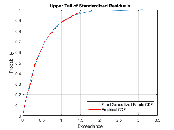
Although the previous graph illustrates the composite CDF, it is instructive to examine the GPD fit in more detail.

The CDF of a GP distribution is parameterized as

for exceedances (y), tail index parameter (zeta), and scale parameter (beta).

To visually assess the GPD fit, plot the empirical CDF of the upper tail exceedances of the residuals along with the CDF fitted by the GPD. Although only 10% of the standardized residuals is used, the fitted distribution closely follows the exceedance data, so the GPD model seems to be a good choice.

figure
[P,Q] = boundary(tails{index});  % cumulative probabilities & quantiles at boundaries
y     = sort(residuals(residuals(:,index) > Q(2), index) - Q(2)); % sort exceedances
plot(y, (cdf(tails{index}, y + Q(2)) - P(2))/P(1))
[F,x] = ecdf(y);                 % empirical CDF
hold on
stairs(x, F, 'r')
grid on

legend('Fitted Generalized Pareto CDF','Empirical CDF','Location','SouthEast');
xlabel('Exceedance')
ylabel('Probability')
title('Upper Tail of Standardized Residuals')

Calibrate the t Copula

Given the standardized residuals, now estimate the scalar degrees of freedom parameter (DoF) and the linear correlation matrix (R) of the t copula using the copulafit function found in the Statistics and Machine Learning Toolbox. The copulafit function allows users to estimate the parameters of the t copula by two distinct methods.

The default method is a formal maximum likelihood approach performed in a two-step process.

Specifically, although the full log-likelihood could be maximized directly, the maximum of the objective function often occurs in a long, flat, narrow valley in multi-dimensional space, and convergence difficulties may arise in high dimensions. To circumvent these difficulties, copulafit performs the maximum likelihood estimation (MLE) in two steps. The inner step maximizes the log-likelihood with respect to the linear correlation matrix, given a fixed value for the degrees of freedom. That conditional maximization is placed within a 1-D maximization with respect to the degrees of freedom, thus maximizing the log-likelihood over all parameters. The function being maximized in this outer step is known as the profile log-likelihood for the degrees of freedom.

In contrast, the following code segment uses an alternative which approximates the profile log-likelihood for the degrees of freedom parameter for large sample sizes. Although this method is often significantly faster than MLE, it should be used with caution because the estimates and confidence limits may not be accurate for small or moderate sample sizes.

Specifically, the approximation is derived by differentiating the log-likelihood function with respect to the linear correlation matrix, assuming the degrees of freedom is a fixed constant. The resulting non-linear equation is then solved iteratively for the correlation matrix. This iteration is, in turn, nested within another optimization to estimate the degrees of freedom. This method is similar in spirit to the profile log-likelihood method above, but is not a true MLE in that the correlation matrix does not converge to the conditional MLE for a given degrees of freedom. However, for large sample sizes the estimates are often quite close to the MLE (see [1] and [7]).

Yet another method estimates the linear correlation matrix by first computing the sample rank correlation matrix (Kendall's tau or Spearman's rho), then converts the rank correlation to a linear correlation with a robust sine transformation. Given this estimate of the linear correlation matrix, the log-likelihood function is then maximized with respect to the degrees of freedom parameter alone. This method also seems motivated by the profile log-likelihood approach, but is not an MLE method at all. However, this method does not require matrix inversion and therefore has the advantage of being numerically stable in the presence of close-to-singular correlation matrices (see [8]).

Finally, Nystrom and Skoglund [6] propose reserving the degrees of freedom parameter as a user-specified simulation input, thus allowing the user to subjectively induce the extent of tail dependence between assets. In particular, they recommend a relatively low degrees of freedom, somewhere between 1 and 2, thus allowing a closer examination of the likelihood of joint extremes. This method is useful for stress testing in which the degree of extreme codependence is of critical importance.

The code segment below first transforms the standardized residuals to uniform variates by the semi-parametric empirical CDF derived above, then fits the t copula to the transformed data. When the uniform variates are transformed by the empirical CDF of each margin, the calibration method is often known as canonical maximum likelihood (CML).

U = zeros(size(residuals));

for i = 1:nIndices
    U(:,i) = cdf(tails{i}, residuals(:,i)); % transform margin to uniform
end

[R, DoF] = copulafit('t', U, 'Method', 'approximateml'); % fit the copula

Simulate Global Index Portfolio Returns with a t Copula

Given the parameters of a t copula, now simulate jointly dependent equity index returns by first simulating the corresponding dependent standardized residuals.

To do so, first simulate dependent uniform variates using the copularnd function found in the Statistics and Machine Learning Toolbox.

Then, by extrapolating into the GP tails and interpolating into the smoothed interior, transform the uniform variates to standardized residuals via the inversion of the semi-parametric marginal CDF of each index. This produces simulated standardized residuals consistent with those obtained from the AR(1) + GJR(1,1) filtering process above. These residuals are independent in time but dependent at any point in time. Each column of the simulated standardized residuals array represents an i.i.d. univariate stochastic process when viewed in isolation, whereas each row shares the rank correlation induced by the copula.

The following code segment simulates 2000 independent random trials of dependent standardized index residuals over a one month horizon of 22 trading days.

s = RandStream.getGlobalStream();
reset(s)

nTrials = 2000;                                   % # of independent random trials
horizon = 22;                                     % VaR forecast horizon

Z = zeros(horizon, nTrials, nIndices);            % standardized residuals array
U = copularnd('t', R, DoF, horizon * nTrials);    % t copula simulation

for j = 1:nIndices
    Z(:,:,j) = reshape(icdf(tails{j}, U(:,j)), horizon, nTrials);
end

Using the simulated standardized residuals as the i.i.d. input noise process, reintroduce the autocorrelation and heteroskedasticity observed in the original index returns via the Econometrics Toolbox™ filter function.

Note that filter accepts user-specified standardized disturbances derived from the copula and simulates multiple paths for a single index model at a time, which means that all sample paths are simulated and stored for each index in succession.

To make the most of current information, specify the necessary presample model residuals, variances, and returns so that each simulated path evolves from a common initial state.

Y0 = returns(end,:);                    % presample returns
Z0 = residuals(end,:);                  % presample standardized residuals
V0 = variances(end,:);                  % presample variances

simulatedReturns = zeros(horizon, nTrials, nIndices);

for i = 1:nIndices
    simulatedReturns(:,:,i) = filter(fit{i}, Z(:,:,i), ...
                                    'Y0', Y0(i), 'Z0', Z0(i), 'V0', V0(i));
end

Now reshape the simulated returns array such that each page represents a single trial of a multivariate return series, rather than multiple trials of a univariate return series.

simulatedReturns = permute(simulatedReturns, [1 3 2]);

Finally, given the simulated returns of each index, form an equally weighted global index portfolio composed of the individual indices (a global index of country indices). Since we are working with daily logarithmic returns, the cumulative returns over the risk horizon are simply the sums of the returns over each intervening period. Also note that the portfolio weights are held fixed throughout the risk horizon, and that the simulation ignores any transaction costs required to rebalance the portfolio (the daily rebalancing process is assumed to be self-financing).

Note that although the simulated returns are logarithmic (continuously compounded), the portfolio return series is constructed by first converting the individual logarithmic returns to arithmetic returns (price change divided by initial price), then weighting the individual arithmetic returns to obtain the arithmetic return of the portfolio, and finally converting back to portfolio logarithmic return. With daily data and a short VaR horizon, the repeated conversions make little difference, but for longer time periods the disparity may be significant.

cumulativeReturns = zeros(nTrials, 1);
weights           = repmat(1/nIndices, nIndices, 1); % equally weighted portfolio

for i = 1:nTrials
    cumulativeReturns(i) = sum(log(1 + (exp(simulatedReturns(:,:,i)) - 1) * weights));
end

Summarize the Results

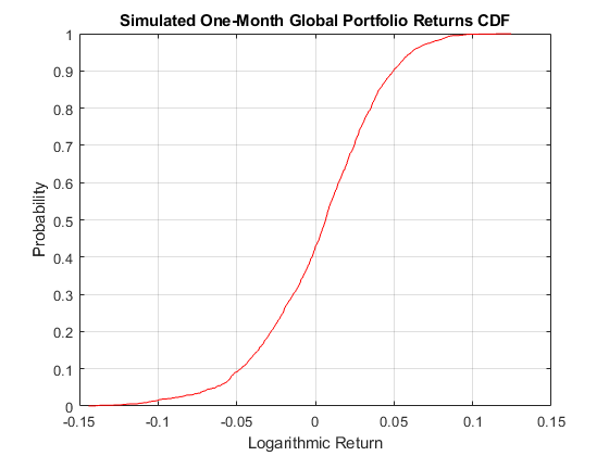
Having simulated the returns of each index and formed the global portfolio, report the maximum gain and loss, as well the VaR at various confidence levels, over the one month risk horizon. Also, plot the empirical CDF of the global portfolio.

VaR = 100 * quantile(cumulativeReturns, [0.10 0.05 0.01]');

disp(' ')
fprintf('Maximum Simulated Loss: %8.4f%s\n'   , -100*min(cumulativeReturns), '%')
fprintf('Maximum Simulated Gain: %8.4f%s\n\n' ,  100*max(cumulativeReturns), '%')
fprintf('     Simulated 90%% VaR: %8.4f%s\n'  ,  VaR(1), '%')
fprintf('     Simulated 95%% VaR: %8.4f%s\n'  ,  VaR(2), '%')
fprintf('     Simulated 99%% VaR: %8.4f%s\n\n',  VaR(3), '%')

figure
h = cdfplot(cumulativeReturns);
h.Color = 'Red';
xlabel('Logarithmic Return')
ylabel('Probability')
title ('Simulated One-Month Global Portfolio Returns CDF')

 
Maximum Simulated Loss:  14.4191%
Maximum Simulated Gain:  12.3974%

     Simulated 90% VaR:  -4.6333%
     Simulated 95% VaR:  -6.3246%
     Simulated 99% VaR: -10.6575%

References

[1] Bouye, E., V. Durrleman, A. Nikeghbali, G. Riboulet, and Roncalli, T. "Copulas for Finance: A Reading Guide and Some Applications." Groupe de Rech. Oper., Credit Lyonnais, Paris, 2000.
[2] Embrechts, P., A. McNeil, and D. Straumann. "Correlation and Dependence in Risk Management: Properties and Pitfalls". Risk Management: Value At Risk and Beyond. Cambridge: Cambridge University Press, 1999, pp. 176–223.
[3] Glosten, L. R., R. Jagannathan, and D. E. Runkle. “On the Relation between the Expected Value and the Volatility of the Nominal Excess Return on Stocks.” The Journal of Finance. Vol. 48, No. 5, 1993, pp. 1779–1801.
[4] McNeil, A. and R. Frey. "Estimation of Tail Related Risk Measure for Heteroscedastic Financial Time Series: An Extreme Value Approach." Journal of Empirical Finance. Vol. 7, 2000, pp. 271–300.
[5] Nystrom, K. and J. Skoglund. "Univariate Extreme Value Theory, GARCH and Measures of Risk." Preprint, submitted 2002.
[6] Nystrom, K. and J. Skoglund. "A Framework for Scenario-Based Risk Management." Preprint, submitted 2002.
[7] Roncalli, T., A. Durrleman, and A. Nikeghbali. "Which Copula Is the Right One?" Groupe de Rech. Oper., Credit Lyonnais, Paris, 2000.
[8] Mashal, R. and A. Zeevi. "Beyond Correlation: Extreme Co-movements between Financial Assets." Columbia University, New York, 2002.