Step 1. Specify a GJR model.

Specify a GJR(1,1) model without a mean offset and $$\kappa =0.1$$, $${\gamma }_1=0.7$$, $${\alpha }_1=0.2$$ and $${\xi }_1=0.1$$.

Mdl = gjr('Constant',0.1,'GARCH',0.7,...
    'ARCH',0.2,'Leverage',0.1);

Step 2. Generate MMSE forecasts.

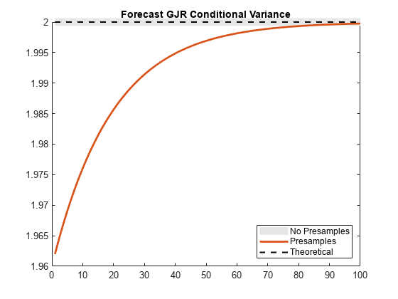
Generate forecasts for a 100-period horizon with and without specifying a presample innovation and conditional variance. Plot the forecasts along with the theoretical unconditional variance of the model.

v1 = forecast(Mdl,100);
v2 = forecast(Mdl,100,'Y0',1.4,'V0',2.1);
denom = 1-Mdl.GARCH{1}-Mdl.ARCH{1}-0.5*Mdl.Leverage{1};
sig2 = Mdl.Constant/denom;

figure
plot(v1,'Color',[.9,.9,.9],'LineWidth',8)
hold on
plot(v2,'LineWidth',2)
plot(ones(100,1)*sig2,'k--','LineWidth',1.5)
xlim([0,100])
title('Forecast GJR Conditional Variance')
legend('No Presamples','Presamples','Theoretical',...
        'Location','SouthEast')
hold off

v2(1) % Display forecasted conditional variance

ans = 1.9620

The forecasts generated without using presample data are equal to the theoretical unconditional variance. In the absence of presample data, forecast uses the unconditional variance for any required presample innovations and conditional variances.

In this example, for the given presample innovation and conditional variance, the starting forecast is

The leverage term is not included in the forecast since the presample innovation was positive (thus, the negative-innovation indicator is zero).