Load Data

Unzip and load the new images as an image datastore. imageDatastore automatically labels the images based on folder names and stores the data as an ImageDatastore object. An image datastore enables you to store large image data, including data that does not fit in memory, and efficiently read batches of images during training of a convolutional neural network.

unzip('MerchData.zip');
imds = imageDatastore('MerchData', ...
    'IncludeSubfolders',true, ...
    'LabelSource','foldernames');

Divide the data into training and validation data sets. Use 70% of the images for training and 30% for validation. splitEachLabel splits the image datastore into two new datastores.

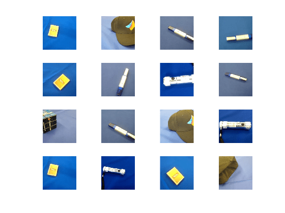
[imdsTrain,imdsValidation] = splitEachLabel(imds,0.7,'randomized');

This very small data set now contains 55 training images and 20 validation images. Display some sample images.

numTrainImages = numel(imdsTrain.Labels);
idx = randperm(numTrainImages,16);
figure
for i = 1:16
    subplot(4,4,i)
    I = readimage(imdsTrain,idx(i));
    imshow(I)
end

Load Pretrained Network

Load the pretrained GoogLeNet neural network. If Deep Learning Toolbox™ Model for GoogLeNet Network is not installed, then the software provides a download link.

net = googlenet;

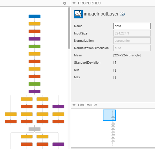
Use deepNetworkDesigner to display an interactive visualization of the network architecture and detailed information about the network layers.

deepNetworkDesigner(net)

The first layer, which is the image input layer, requires input images of size 224-by-224-by-3, where 3 is the number of color channels.

inputSize = net.Layers(1).InputSize

inputSize = 1×3

   224   224     3

Replace Final Layers

The fully connected layer and classification layer of the pretrained network net are configured for 1000 classes. These two layers, loss3-classifier and output in GoogLeNet, contain information on how to combine the features that the network extracts into class probabilities, a loss value, and predicted labels. To retrain a pretrained network to classify new images, replace these two layers with new layers adapted to the new data set.

Extract the layer graph from the trained network.

lgraph = layerGraph(net); 

Replace the fully connected layer with a new fully connected layer that has number of outputs equal to the number of classes. To make learning faster in the new layers than in the transferred layers, increase the WeightLearnRateFactor and BiasLearnRateFactor values of the fully connected layer.

numClasses = numel(categories(imdsTrain.Labels))

numClasses = 5

newLearnableLayer = fullyConnectedLayer(numClasses, ...
    'Name','new_fc', ...
    'WeightLearnRateFactor',10, ...
    'BiasLearnRateFactor',10);
    
lgraph = replaceLayer(lgraph,'loss3-classifier',newLearnableLayer);

The classification layer specifies the output classes of the network. Replace the classification layer with a new one without class labels. trainNetwork automatically sets the output classes of the layer at training time.

newClassLayer = classificationLayer('Name','new_classoutput');
lgraph = replaceLayer(lgraph,'output',newClassLayer);

Train Network

The network requires input images of size 224-by-224-by-3, but the images in the image datastores have different sizes. Use an augmented image datastore to automatically resize the training images. Specify additional augmentation operations to perform on the training images: randomly flip the training images along the vertical axis, and randomly translate them up to 30 pixels horizontally and vertically. Data augmentation helps prevent the network from overfitting and memorizing the exact details of the training images.

pixelRange = [-30 30];
imageAugmenter = imageDataAugmenter( ...
    'RandXReflection',true, ...
    'RandXTranslation',pixelRange, ...
    'RandYTranslation',pixelRange);
augimdsTrain = augmentedImageDatastore(inputSize(1:2),imdsTrain, ...
    'DataAugmentation',imageAugmenter);

To automatically resize the validation images without performing further data augmentation, use an augmented image datastore without specifying any additional preprocessing operations.

augimdsValidation = augmentedImageDatastore(inputSize(1:2),imdsValidation);

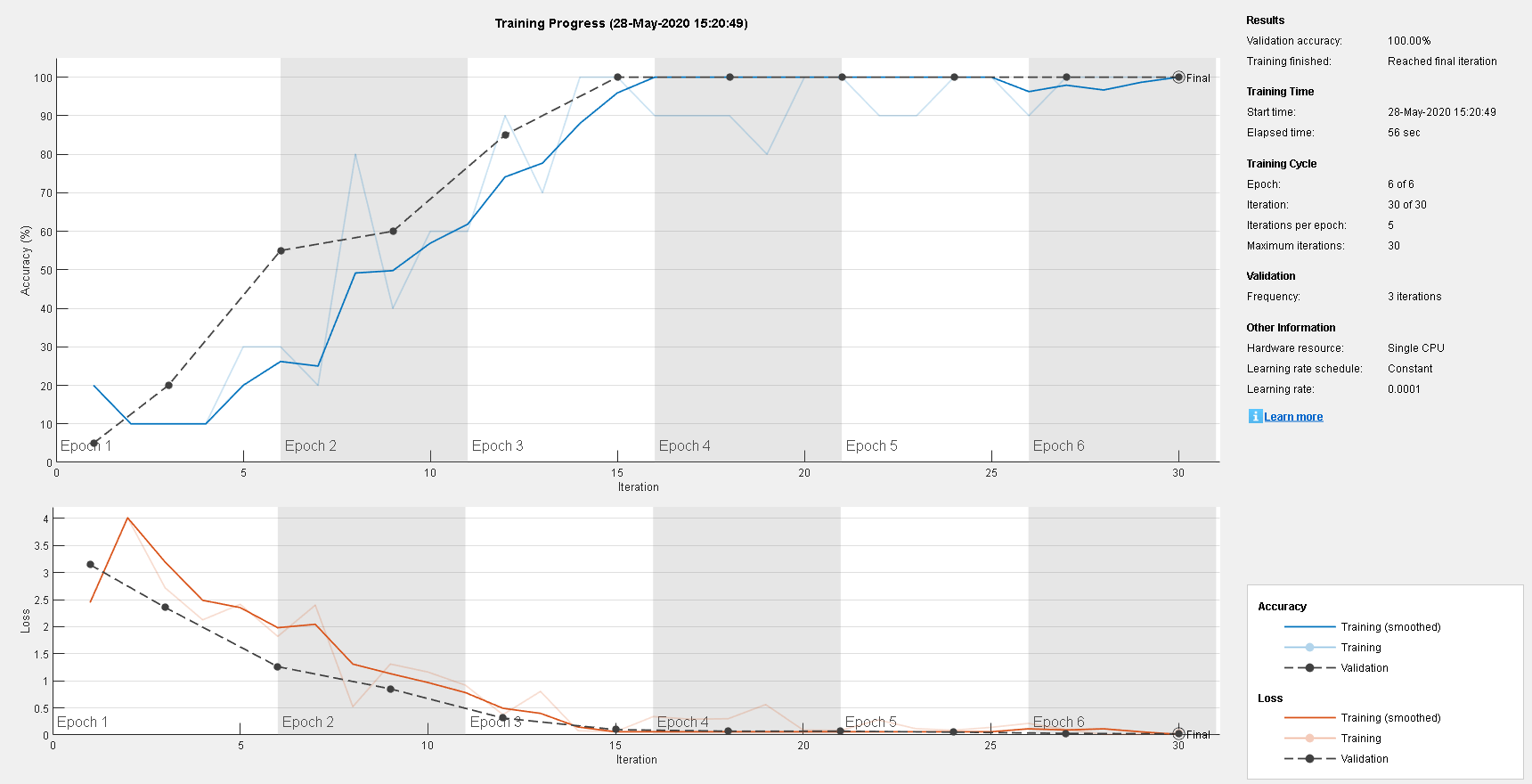
Specify the training options. For transfer learning, keep the features from the early layers of the pretrained network (the transferred layer weights). To slow down learning in the transferred layers, set the initial learning rate to a small value. In the previous step, you increased the learning rate factors for the fully connected layer to speed up learning in the new final layers. This combination of learning rate settings results in fast learning only in the new layers and slower learning in the other layers. When performing transfer learning, you do not need to train for as many epochs. An epoch is a full training cycle on the entire training data set. Specify the mini-batch size and validation data. The software validates the network every ValidationFrequency iterations during training.

options = trainingOptions('sgdm', ...
    'MiniBatchSize',10, ...
    'MaxEpochs',6, ...
    'InitialLearnRate',1e-4, ...
    'Shuffle','every-epoch', ...
    'ValidationData',augimdsValidation, ...
    'ValidationFrequency',3, ...
    'Verbose',false, ...
    'Plots','training-progress');

Train the network consisting of the transferred and new layers. By default, trainNetwork uses a GPU if one is available. This requires Parallel Computing Toolbox™ and a supported GPU device. For information on supported devices, see GPU Computing Requirements (Parallel Computing Toolbox). Otherwise, it uses a CPU. You can also specify the execution environment by using the 'ExecutionEnvironment' name-value pair argument of trainingOptions.

netTransfer = trainNetwork(augimdsTrain,lgraph,options);

Classify Validation Images

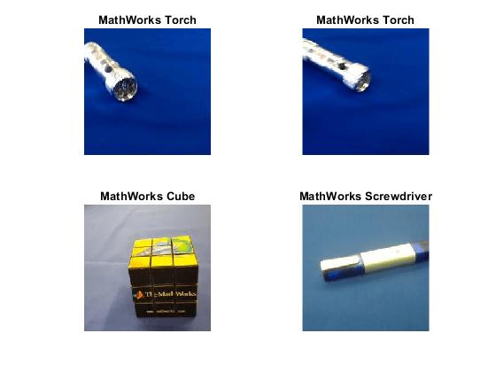
Classify the validation images using the fine-tuned network.

[YPred,scores] = classify(netTransfer,augimdsValidation);

Display four sample validation images with their predicted labels.

idx = randperm(numel(imdsValidation.Files),4);
figure
for i = 1:4
    subplot(2,2,i)
    I = readimage(imdsValidation,idx(i));
    imshow(I)
    label = YPred(idx(i));
    title(string(label));
end

Calculate the classification accuracy on the validation set. Accuracy is the fraction of labels that the network predicts correctly.

YValidation = imdsValidation.Labels;
accuracy = mean(YPred == YValidation)

accuracy = 1

For tips on improving classification accuracy, see Deep Learning Tips and Tricks.

References

[1] Krizhevsky, Alex, Ilya Sutskever, and Geoffrey E. Hinton. "ImageNet Classification with Deep Convolutional Neural Networks." Advances in neural information processing systems 25 (2012).
[2] Szegedy, Christian, Wei Liu, Yangqing Jia, Pierre Sermanet, Scott Reed, Dragomir Anguelov, Dumitru Erhan, Vincent Vanhoucke, and Andrew Rabinovich. "Going deeper with convolutions." Proceedings of the IEEE conference on computer vision and pattern recognition (2015): 1–9.
[3] "BVLC GoogLeNet Model." https://github.com/BVLC/caffe/tree/master/models/bvlc_googlenet.
See Also
trainNetwork | trainingOptions | squeezenet | googlenet | analyzeNetwork | Deep Network