Load Data

Unzip and load the new images as an image datastore. This very small data set contains only 75 images. Divide the data into training and validation data sets. Use 70% of the images for training and 30% for validation.

unzip('MerchData.zip');
imds = imageDatastore('MerchData', ...
    'IncludeSubfolders',true, ...
    'LabelSource','foldernames'); 
[imdsTrain,imdsValidation] = splitEachLabel(imds,0.7);

Load Pretrained Network

Load a pretrained GoogLeNet network. If the Deep Learning Toolbox™ Model for GoogLeNet Network support package is not installed, then the software provides a download link.

To try a different pretrained network, open this example in MATLAB® and select a different network. For example, you can try squeezenet, a network that is even faster than googlenet. You can run this example with other pretrained networks. For a list of all available networks, see Load Pretrained Neural Networks.

net = googlenet;

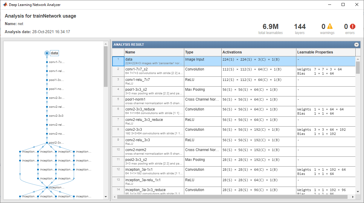
Use analyzeNetwork to display an interactive visualization of the network architecture and detailed information about the network layers.

analyzeNetwork(net)

The first element of the Layers property of the network is the image input layer. For a GoogLeNet network, this layer requires input images of size 224-by-224-by-3, where 3 is the number of color channels. Other networks can require input images with different sizes. For example, the Xception network requires images of size 299-by-299-by-3.

net.Layers(1)

ans = 
  ImageInputLayer with properties:

                      Name: 'data'
                 InputSize: [224 224 3]

   Hyperparameters
          DataAugmentation: 'none'
             Normalization: 'zerocenter'
    NormalizationDimension: 'auto'
                      Mean: [224×224×3 single]

inputSize = net.Layers(1).InputSize;

Replace Final Layers

The convolutional layers of the network extract image features that the last learnable layer and the final classification layer use to classify the input image. These two layers, 'loss3-classifier' and 'output' in GoogLeNet, contain information on how to combine the features that the network extracts into class probabilities, a loss value, and predicted labels. To retrain a pretrained network to classify new images, replace these two layers with new layers adapted to the new data set.

Convert the trained network to a layer graph.

lgraph = layerGraph(net);

Find the names of the two layers to replace. You can do this manually or you can use the supporting function findLayersToReplace to find these layers automatically.

[learnableLayer,classLayer] = findLayersToReplace(lgraph);
[learnableLayer,classLayer] 

ans = 
  1×2 Layer array with layers:

     1   'loss3-classifier'   Fully Connected         1000 fully connected layer
     2   'output'             Classification Output   crossentropyex with 'tench' and 999 other classes

In most networks, the last layer with learnable weights is a fully connected layer. Replace this fully connected layer with a new fully connected layer with the number of outputs equal to the number of classes in the new data set (5, in this example). In some networks, such as SqueezeNet, the last learnable layer is a 1-by-1 convolutional layer instead. In this case, replace the convolutional layer with a new convolutional layer with the number of filters equal to the number of classes. To learn faster in the new layer than in the transferred layers, increase the learning rate factors of the layer.

numClasses = numel(categories(imdsTrain.Labels));

if isa(learnableLayer,'nnet.cnn.layer.FullyConnectedLayer')
    newLearnableLayer = fullyConnectedLayer(numClasses, ...
        'Name','new_fc', ...
        'WeightLearnRateFactor',10, ...
        'BiasLearnRateFactor',10);
    
elseif isa(learnableLayer,'nnet.cnn.layer.Convolution2DLayer')
    newLearnableLayer = convolution2dLayer(1,numClasses, ...
        'Name','new_conv', ...
        'WeightLearnRateFactor',10, ...
        'BiasLearnRateFactor',10);
end

lgraph = replaceLayer(lgraph,learnableLayer.Name,newLearnableLayer);

The classification layer specifies the output classes of the network. Replace the classification layer with a new one without class labels. trainNetwork automatically sets the output classes of the layer at training time.

newClassLayer = classificationLayer('Name','new_classoutput');
lgraph = replaceLayer(lgraph,classLayer.Name,newClassLayer);

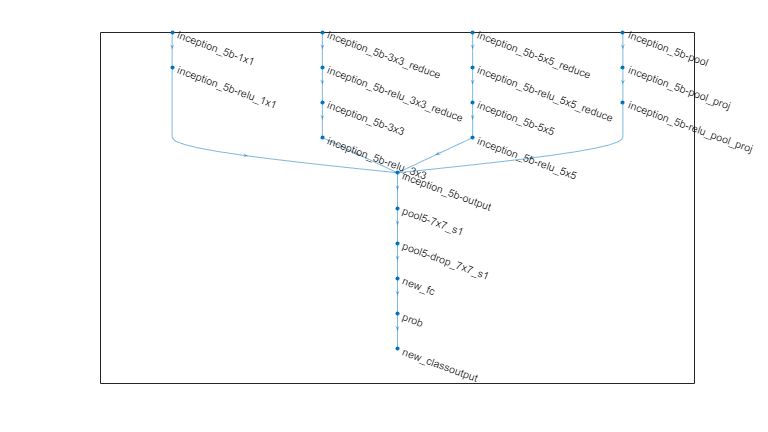
To check that the new layers are connected correctly, plot the new layer graph and zoom in on the last layers of the network.

figure('Units','normalized','Position',[0.3 0.3 0.4 0.4]);
plot(lgraph)
ylim([0,10])

Freeze Initial Layers

The network is now ready to be retrained on the new set of images. Optionally, you can "freeze" the weights of earlier layers in the network by setting the learning rates in those layers to zero. During training, trainNetwork does not update the parameters of the frozen layers. Because the gradients of the frozen layers do not need to be computed, freezing the weights of many initial layers can significantly speed up network training. If the new data set is small, then freezing earlier network layers can also prevent those layers from overfitting to the new data set.

Extract the layers and connections of the layer graph and select which layers to freeze. In GoogLeNet, the first 10 layers make out the initial 'stem' of the network. Use the supporting function freezeWeights to set the learning rates to zero in the first 10 layers. Use the supporting function createLgraphUsingConnections to reconnect all the layers in the original order. The new layer graph contains the same layers, but with the learning rates of the earlier layers set to zero.

layers = lgraph.Layers;
connections = lgraph.Connections;

layers(1:10) = freezeWeights(layers(1:10));
lgraph = createLgraphUsingConnections(layers,connections);

Train Network

The network requires input images of size 224-by-224-by-3, but the images in the image datastore have different sizes. Use an augmented image datastore to automatically resize the training images. Specify additional augmentation operations to perform on the training images: randomly flip the training images along the vertical axis and randomly translate them up to 30 pixels and scale them up to 10% horizontally and vertically. Data augmentation helps prevent the network from overfitting and memorizing the exact details of the training images.

pixelRange = [-30 30];
scaleRange = [0.9 1.1];
imageAugmenter = imageDataAugmenter( ...
    'RandXReflection',true, ...
    'RandXTranslation',pixelRange, ...
    'RandYTranslation',pixelRange, ...
    'RandXScale',scaleRange, ...
    'RandYScale',scaleRange);
augimdsTrain = augmentedImageDatastore(inputSize(1:2),imdsTrain, ...
    'DataAugmentation',imageAugmenter);

To automatically resize the validation images without performing further data augmentation, use an augmented image datastore without specifying any additional preprocessing operations.

augimdsValidation = augmentedImageDatastore(inputSize(1:2),imdsValidation);

Specify the training options. Set InitialLearnRate to a small value to slow down learning in the transferred layers that are not already frozen. In the previous step, you increased the learning rate factors for the last learnable layer to speed up learning in the new final layers. This combination of learning rate settings results in fast learning in the new layers, slower learning in the middle layers, and no learning in the earlier, frozen layers.

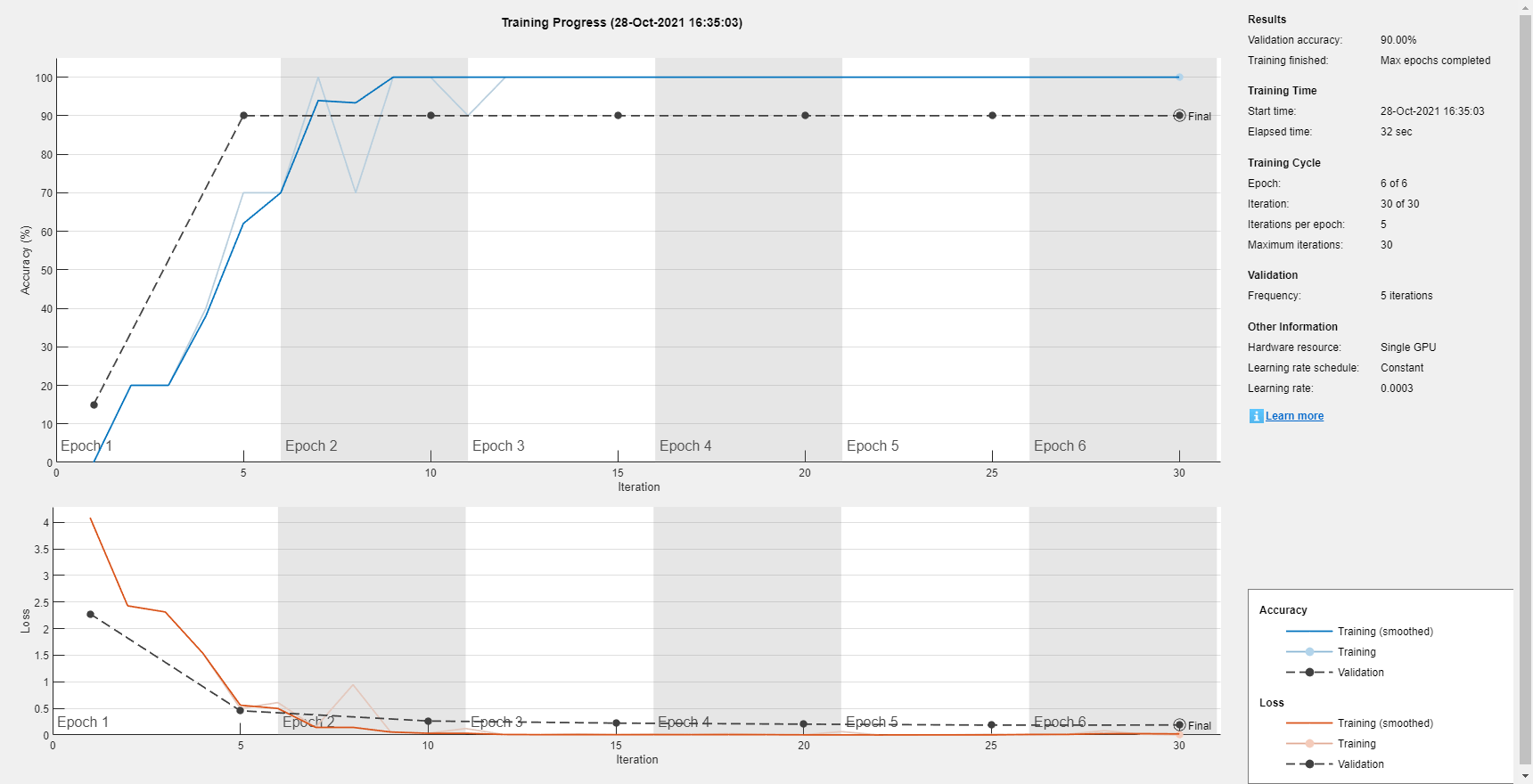
Specify the number of epochs to train for. When performing transfer learning, you do not need to train for as many epochs. An epoch is a full training cycle on the entire training data set. Specify the mini-batch size and validation data. Compute the validation accuracy once per epoch.

miniBatchSize = 10;
valFrequency = floor(numel(augimdsTrain.Files)/miniBatchSize);
options = trainingOptions('sgdm', ...
    'MiniBatchSize',miniBatchSize, ...
    'MaxEpochs',6, ...
    'InitialLearnRate',3e-4, ...
    'Shuffle','every-epoch', ...
    'ValidationData',augimdsValidation, ...
    'ValidationFrequency',valFrequency, ...
    'Verbose',false, ...
    'Plots','training-progress');

Train the network using the training data. By default, trainNetwork uses a GPU if one is available. This requires Parallel Computing Toolbox™ and a supported GPU device. For information on supported devices, see GPU Computing Requirements (Parallel Computing Toolbox). Otherwise, trainNetwork uses a CPU. You can also specify the execution environment by using the 'ExecutionEnvironment' name-value pair argument of trainingOptions. Because the data set is so small, training is fast.

net = trainNetwork(augimdsTrain,lgraph,options);

Classify Validation Images

Classify the validation images using the fine-tuned network, and calculate the classification accuracy.

[YPred,probs] = classify(net,augimdsValidation);
accuracy = mean(YPred == imdsValidation.Labels)

accuracy = 0.9000

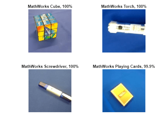
Display four sample validation images with predicted labels and the predicted probabilities of the images having those labels.

idx = randperm(numel(imdsValidation.Files),4);
figure
for i = 1:4
    subplot(2,2,i)
    I = readimage(imdsValidation,idx(i));
    imshow(I)
    label = YPred(idx(i));
    title(string(label) + ", " + num2str(100*max(probs(idx(i),:)),3) + "%");
end