Load Data

Unzip and load the sample images as an image datastore. imageDatastore automatically labels the images based on folder names and stores the data as an ImageDatastore object. An image datastore lets you store large image data, including data that does not fit in memory. Split the data into 70% training and 30% test data.

unzip('MerchData.zip');
imds = imageDatastore('MerchData','IncludeSubfolders',true,'LabelSource','foldernames');
[imdsTrain,imdsTest] = splitEachLabel(imds,0.7,'randomized');

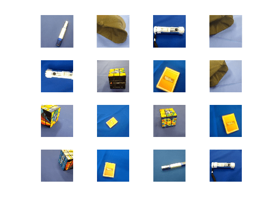
There are now 55 training images and 20 validation images in this very small data set. Display some sample images.

numTrainImages = numel(imdsTrain.Labels);
idx = randperm(numTrainImages,16);
figure
for i = 1:16
    subplot(4,4,i)
    I = readimage(imdsTrain,idx(i));
    imshow(I)
end

Load Pretrained Network

Load a pretrained ResNet-18 network. If the Deep Learning Toolbox Model for ResNet-18 Network support package is not installed, then the software provides a download link. ResNet-18 is trained on more than a million images and can classify images into 1000 object categories, such as keyboard, mouse, pencil, and many animals. As a result, the model has learned rich feature representations for a wide range of images.

net = resnet18

net = 
  DAGNetwork with properties:

         Layers: [71x1 nnet.cnn.layer.Layer]
    Connections: [78x2 table]
     InputNames: {'data'}
    OutputNames: {'ClassificationLayer_predictions'}

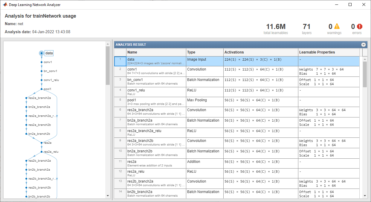
Analyze the network architecture. The first layer, the image input layer, requires input images of size 224-by-224-by-3, where 3 is the number of color channels.

inputSize = net.Layers(1).InputSize;
analyzeNetwork(net)

Extract Image Features

The network requires input images of size 224-by-224-by-3, but the images in the image datastores have different sizes. To automatically resize the training and test images before they are input to the network, create augmented image datastores, specify the desired image size, and use these datastores as input arguments to activations.

augimdsTrain = augmentedImageDatastore(inputSize(1:2),imdsTrain);
augimdsTest = augmentedImageDatastore(inputSize(1:2),imdsTest);

The network constructs a hierarchical representation of input images. Deeper layers contain higher-level features, constructed using the lower-level features of earlier layers. To get the feature representations of the training and test images, use activations on the global pooling layer, 'pool5', at the end of the network. The global pooling layer pools the input features over all spatial locations, giving 512 features in total.

layer = 'pool5';
featuresTrain = activations(net,augimdsTrain,layer,'OutputAs','rows');
featuresTest = activations(net,augimdsTest,layer,'OutputAs','rows');

whos featuresTrain

  Name                Size              Bytes  Class     Attributes

  featuresTrain      55x512            112640  single              

Extract the class labels from the training and test data.

YTrain = imdsTrain.Labels;
YTest = imdsTest.Labels;

Fit Image Classifier

Use the features extracted from the training images as predictor variables and fit a multiclass support vector machine (SVM) using fitcecoc (Statistics and Machine Learning Toolbox).

classifier = fitcecoc(featuresTrain,YTrain);

Classify Test Images

Classify the test images using the trained SVM model using the features extracted from the test images.

YPred = predict(classifier,featuresTest);

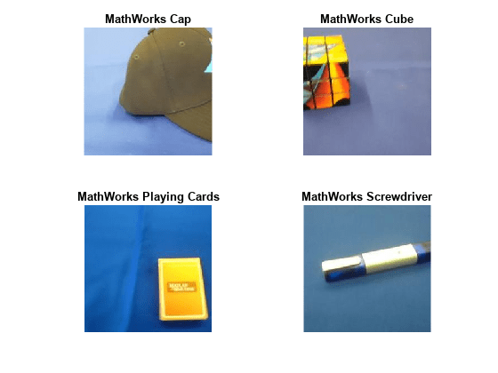
Display four sample test images with their predicted labels.

idx = [1 5 10 15];
figure
for i = 1:numel(idx)
    subplot(2,2,i)
    I = readimage(imdsTest,idx(i));
    label = YPred(idx(i));
    imshow(I)
    title(char(label))
end

Calculate the classification accuracy on the test set. Accuracy is the fraction of labels that the network predicts correctly.

accuracy = mean(YPred == YTest)

accuracy = 1

Train Classifier on Shallower Features

You can also extract features from an earlier layer in the network and train a classifier on those features. Earlier layers typically extract fewer, shallower features, have higher spatial resolution, and a larger total number of activations. Extract the features from the 'res3b_relu' layer. This is the final layer that outputs 128 features and the activations have a spatial size of 28-by-28.

layer = 'res3b_relu';
featuresTrain = activations(net,augimdsTrain,layer);
featuresTest = activations(net,augimdsTest,layer);
whos featuresTrain

  Name                Size                      Bytes  Class     Attributes

  featuresTrain      28x28x128x55            22077440  single              

The extracted features used in the first part of this example were pooled over all spatial locations by the global pooling layer. To achieve the same result when extracting features in earlier layers, manually average the activations over all spatial locations. To get the features on the form N-by-C, where N is the number of observations and C is the number of features, remove the singleton dimensions and transpose.

featuresTrain = squeeze(mean(featuresTrain,[1 2]))';
featuresTest = squeeze(mean(featuresTest,[1 2]))';
whos featuresTrain

  Name                Size             Bytes  Class     Attributes

  featuresTrain      55x128            28160  single              

Train an SVM classifier on the shallower features. Calculate the test accuracy.

classifier = fitcecoc(featuresTrain,YTrain);
YPred = predict(classifier,featuresTest);
accuracy = mean(YPred == YTest)

accuracy = 0.9500

Both trained SVMs have high accuracies. If the accuracy is not high enough using feature extraction, then try transfer learning instead. For an example, see Train Deep Learning Network to Classify New Images. For a list and comparison of the pretrained networks, see Pretrained Deep Neural Networks.