Shallow Neural Network Time-Series Prediction and Modeling
Dynamic neural networks are good at time-series prediction. To see examples of using NARX networks being applied in open-loop form, closed-loop form and open/closed-loop multistep prediction, see Multistep Neural Network Prediction.
Tip
For deep learning with time series data, see instead Sequence Classification Using Deep Learning.
Suppose, for instance, that you have data from a pH neutralization process. You want to design a network that can predict the pH of a solution in a tank from past values of the pH and past values of the acid and base flow rate into the tank. You have a total of 2001 time steps for which you have those series.
You can solve this problem in two ways:
Use the Neural Net Time Series app, as described in Fit Time Series Data Using the Neural Net Time Series App.
Use command-line functions, as described in Fit Time Series Data Using Command-Line Functions.
Note
To interactively build, visualize, and train deep learning neural networks, use the Deep Network Designer app. For more information, see Get Started with Deep Network Designer.
It is generally best to start with the app, and then use the app to automatically generate command-line scripts. Before using either method, first define the problem by selecting a data set. Each of the neural network apps has access to several sample data sets that you can use to experiment with the toolbox (see Sample Data Sets for Shallow Neural Networks). If you have a specific problem that you want to solve, you can load your own data into the workspace.
Time Series Networks
You can train a neural network to solve three types of time series problems.
NARX Network
In the first type of time series problem, you would like to predict future values of a time series y(t) from past values of that time series and past values of a second time series x(t). This form of prediction is called nonlinear autoregressive with exogenous (external) input, or NARX (see Design Time Series NARX Feedback Neural Networks), and can be written as follows:
y(t) = f(y(t – 1), ..., y(t – d), x(t – 1), ..., (t – d))
Use this model to predict future values of a stock or bond, based on such economic variables as unemployment rates, GDP, etc. You can also use this model for system identification, in which models are developed to represent dynamic systems, such as chemical processes, manufacturing systems, robotics, aerospace vehicles, etc.
NAR Network
In the second type of time series problem, there is only one series involved. The future values of a time series y(t) are predicted only from past values of that series. This form of prediction is called nonlinear autoregressive, or NAR, and can be written as follows:
y(t) = f(y(t – 1), ..., y(t – d))
You can use this model to predict financial instruments, but without the use of a companion series.
Nonlinear Input-Output Network
The third time series problem is similar to the first type, in that two series are involved, an input series x(t) and an output series y(t). Here you want to predict values of y(t) from previous values of x(t), but without knowledge of previous values of y(t). This input/output model can be written as follows:
y(t) = f(x(t – 1), ..., x(t – d))
The NARX model will provide better predictions than this input-output model, because it uses the additional information contained in the previous values of y(t). However, there may be some applications in which the previous values of y(t) would not be available. Those are the only cases where you would want to use the input-output model instead of the NARX model.
Defining a Problem
To define a time series problem for the toolbox, arrange a set of time series predictor vectors as columns in a cell array. Then, arrange another set of time series response vectors (the correct response vectors for each of the predictor vectors) into a second cell array. Additionally, there are cases in which you only need to have a response data set. For example, you can define the following time series problem, in which you want to use previous values of a series to predict the next value:
responses = {1 2 3 4 5};
The next section shows how to train a network to fit a time series data set, using the Neural Net Time Series app. This example uses example data provided with the toolbox.
Fit Time Series Data Using the Neural Net Time Series App
This example shows how to train a shallow neural network to fit time series data using the Neural Net Time Series app.
Open the Neural Net Time Series app using ntstool.
ntstool
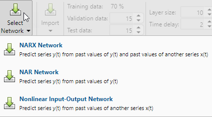
Select Network
You can use the Neural Net Time Series app to solve three different kinds of time series problems.
In the first type of time series problem, you would like to predict future values of a time series from past values of that time series and past values of a second time series . This form of prediction is called nonlinear autoregressive network with exogenous (external) input, or NARX.
In the second type of time series problem, there is only one series involved. The future values of a time series are predicted only from past values of that series. This form of prediction is called nonlinear autoregressive, or NAR.
The third time series problem is similar to the first type, in that two series are involved, an input series (predictors) and an output series (responses) . Here you want to predict values of from previous values of , but without knowledge of previous values of .
For this example, use a NARX network. Click Select Network > NARX Network.
Select Data
The Neural Net Time Series app has example data to help you get started training a neural network.
To import example pH neutralization process data, select Import > More Example Data Sets > Import pH Neutralization Data Set. You can use this data set to train a neural network to predict the pH of a solution using acid and base solution flow. If you import your own data from file or the workspace, you must specify the predictors and responses.
Information about the imported data appears in the Model Summary. This data set contains 2001 time steps. The predictors have two features (acid and base solution flow) and the responses have a single feature (solution pH).
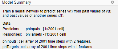
Split the data into training, validation, and test sets. Keep the default settings. The data is split into:
70% for training.
15% to validate that the network is generalizing and to stop training before overfitting.
15% to independently test network generalization.
For more information on data division, see Divide Data for Optimal Neural Network Training.
Create Network
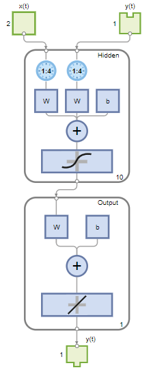
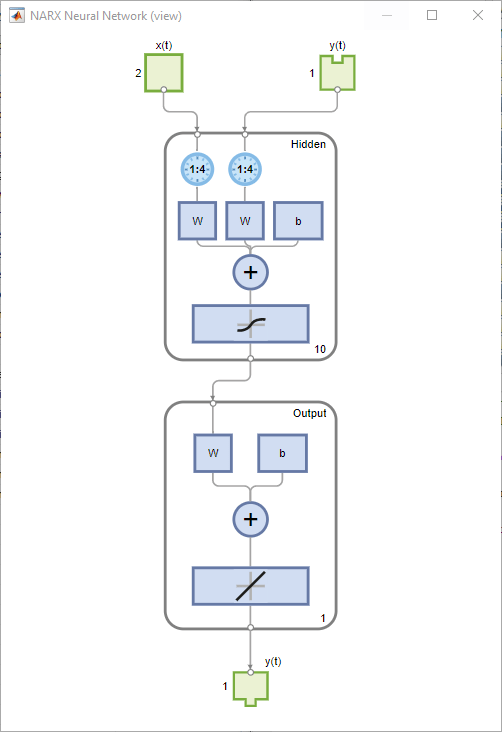
The standard NARX network is a two-layer feedforward network, with a sigmoid transfer function in the hidden layer and a linear transfer function in the output layer. This network also uses tapped delay lines to store previous values of the and sequences. Note that the output of the NARX network, , is fed back to the input of the network (through delays), since is a function of . However, for efficient training this feedback loop can be opened.
Because the true output is available during the training of the network, you can use the open-loop architecture shown below, in which the true output is used instead of feeding back the estimated output. This has two advantages. The first is that the input to the feedforward network is more accurate. The second is that the resulting network has a purely feedforward architecture, and therefore a more efficient algorithm can be used for training. This network is discussed in more detail in Design Time Series NARX Feedback Neural Networks.
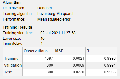
The Layer size value defines the number of hidden neurons. Keep the default layer size, 10. Change the Time delay value to 4. You might want to adjust these numbers if the network training performance is poor.
You can see the network architecture in the Network pane.
Train Network
To train the network, select Train > Train with Levenberg-Marquardt. This is the default training algorithm and the same as clicking Train.
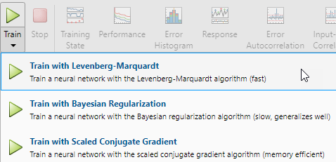
Training with Levenberg-Marquardt (trainlm) is recommended for most problems. For noisy or small problems, Bayesian Regularization (trainbr) can obtain a better solution, at the cost of taking longer. For large problems, Scaled Conjugate Gradient (trainscg) is recommended as it uses gradient calculations which are more memory efficient than the Jacobian calculations the other two algorithms use.
In the Training pane, you can see the training progress. Training continues until one of the stopping criteria is met. In this example, training continues until the validation error increases consecutively for six iterations ("Met validation criterion").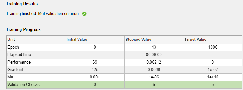
Analyze Results
The Model Summary contains information about the training algorithm and the training results for each data set.
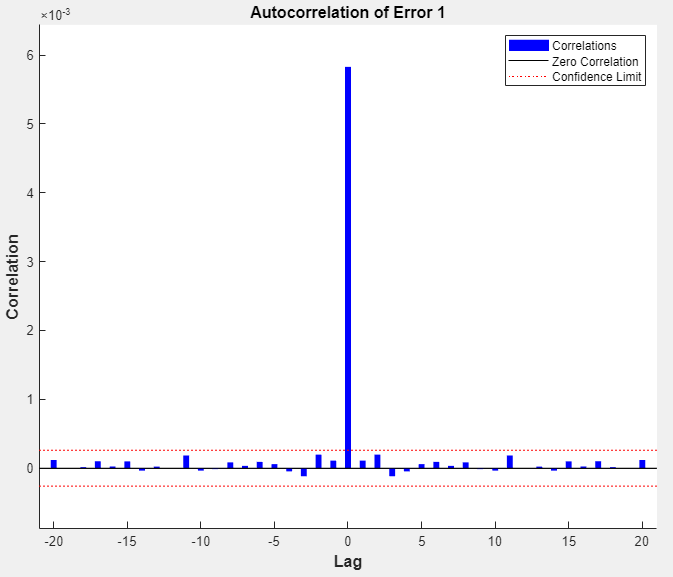
You can further analyze the results by generating plots. To plot the error autocorrelation, in the Plots section, click Error Autocorrelation. The autocorrelation plot describes how the prediction errors are related in time. For a perfect prediction model, there should only be one nonzero value of the autocorrelation function, and it should occur at zero lag (this is the mean square error). This would mean that the prediction errors were completely uncorrelated with each other (white noise). If there was significant correlation in the prediction errors, then it should be possible to improve the prediction - perhaps by increasing the number of delays in the tapped delay lines. In this case, the correlations, except for the one at zero lag, fall approximately within the 95% confidence limits around zero, so the model seems to be adequate. If even more accurate results were required, you could retrain the network. This will change the initial weights and biases of the network, and may produce an improved network after retraining.
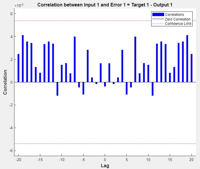
View the input-error cross-correlation plot to obtain additional verification of network performance. In the Plots section, click Input-Error Correlation. The input-error cross-correlation plot illustrates how the errors are correlated with the input sequence . For a perfect prediction model, all of the correlations should be zero. If the input is correlated with the error, then it should be possible to improve the prediction, perhaps by increasing the number of delays in the tapped delay lines. In this case, most of the correlations fall within the confidence bounds around zero.
In the Plots section, click Response. This displays the outputs, responses (targets), and errors versus time. It also indicates which time points were selected for training, testing, and validation.
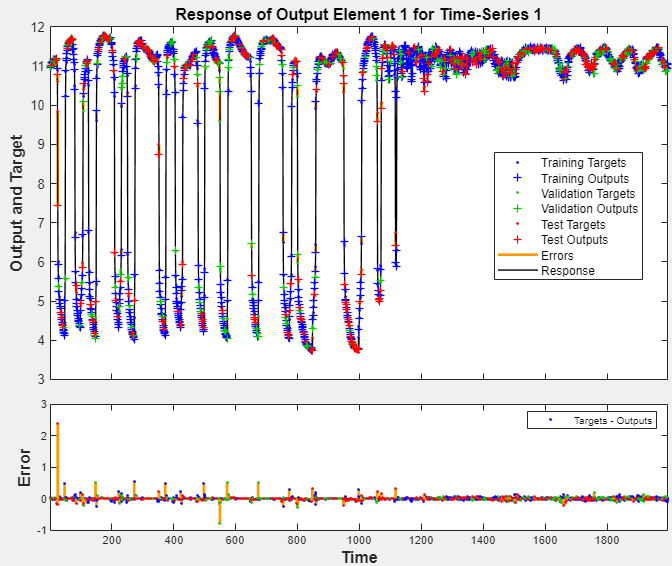
If you are unhappy with the network performance, you can do one of the following:
Train the network again.
Increase the number of hidden neurons.
Use a larger training data set.
If performance on the training set is good but the test set performance is poor, this could indicate the model is overfitting. Decreasing the layer size, and therefore decreasing the number of neurons, can reduce the overfitting.
You can also evaluate the network performance on an additional test set. To load additional test data to evaluate the network with, in the Test section, click Test. The Model Summary displays the additional test data results. You can also generate plots to analyze the additional test data results.
Generate Code
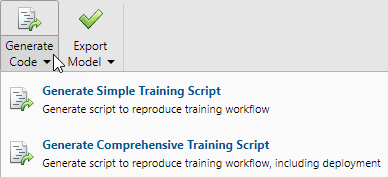
Select Generate Code > Generate Simple Training Script to create MATLAB code to reproduce the previous steps from the command line. Creating MATLAB code can be helpful if you want to learn how to use the command-line functionality of the toolbox to customize the training process. In Fit Time Series Data Using Command-Line Functions, you will investigate the generated scripts in more detail.
Export Network
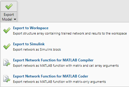
You can export your trained network to the workspace or Simulink®. You can also deploy the network with MATLAB Compiler™ tools and other MATLAB code generation tools. To export your trained network and results, select Export Model > Export to Workspace.
Fit Time Series Data Using Command-Line Functions
The easiest way to learn how to use the command-line functionality of the toolbox is to generate scripts from the apps, and then modify them to customize the network training. As an example, look at the simple script that was generated in the previous section using the Neural Net Time Series app.
% Solve an Autoregression Problem with External Input with a NARX Neural Network
% Script generated by Neural Time Series app
% Created 13-May-2021 17:34:27
%
% This script assumes these variables are defined:
%
%   phInputs - input time series.
%   phTargets - feedback time series.

X = phInputs;
T = phTargets;

% Choose a Training Function
% For a list of all training functions type: help nntrain
% 'trainlm' is usually fastest.
% 'trainbr' takes longer but may be better for challenging problems.
% 'trainscg' uses less memory. Suitable in low memory situations.
trainFcn = 'trainlm';  % Levenberg-Marquardt backpropagation.

% Create a Nonlinear Autoregressive Network with External Input
inputDelays = 1:4;
feedbackDelays = 1:4;
hiddenLayerSize = 10;
net = narxnet(inputDelays,feedbackDelays,hiddenLayerSize,'open',trainFcn);

% Prepare the Data for Training and Simulation
% The function PREPARETS prepares timeseries data for a particular network,
% shifting time by the minimum amount to fill input states and layer
% states. Using PREPARETS allows you to keep your original time series data
% unchanged, while easily customizing it for networks with differing
% numbers of delays, with open loop or closed loop feedback modes.
[x,xi,ai,t] = preparets(net,X,{},T);

% Setup Division of Data for Training, Validation, Testing
net.divideParam.trainRatio = 70/100;
net.divideParam.valRatio = 15/100;
net.divideParam.testRatio = 15/100;

% Train the Network
[net,tr] = train(net,x,t,xi,ai);

% Test the Network
y = net(x,xi,ai);
e = gsubtract(t,y);
performance = perform(net,t,y)

% View the Network
view(net)

% Plots
% Uncomment these lines to enable various plots.
%figure, plotperform(tr)
%figure, plottrainstate(tr)
%figure, ploterrhist(e)
%figure, plotregression(t,y)
%figure, plotresponse(t,y)
%figure, ploterrcorr(e)
%figure, plotinerrcorr(x,e)

% Closed Loop Network
% Use this network to do multi-step prediction.
% The function CLOSELOOP replaces the feedback input with a direct
% connection from the output layer.
netc = closeloop(net);
netc.name = [net.name ' - Closed Loop'];
view(netc)
[xc,xic,aic,tc] = preparets(netc,X,{},T);
yc = netc(xc,xic,aic);
closedLoopPerformance = perform(net,tc,yc)

% Step-Ahead Prediction Network
% For some applications it helps to get the prediction a timestep early.
% The original network returns predicted y(t+1) at the same time it is
% given y(t+1). For some applications such as decision making, it would
% help to have predicted y(t+1) once y(t) is available, but before the
% actual y(t+1) occurs. The network can be made to return its output a
% timestep early by removing one delay so that its minimal tap delay is now
% 0 instead of 1. The new network returns the same outputs as the original
% network, but outputs are shifted left one timestep.
nets = removedelay(net);
nets.name = [net.name ' - Predict One Step Ahead'];
view(nets)
[xs,xis,ais,ts] = preparets(nets,X,{},T);
ys = nets(xs,xis,ais);
stepAheadPerformance = perform(nets,ts,ys)
You can save the script, and then run it from the command line to reproduce the results of the previous app session. You can also edit the script to customize the training process. In this case, follow each of the steps in the script.
Select Data
The script assumes that the predictor and response vectors are already loaded into the workspace. If the data is not loaded, you can load it as follows:
load ph_datasetpHInputs and the responses
pHTargets into the workspace.This data set is one of the sample data sets that is part of the toolbox. For
information about the data sets available, see Sample Data Sets for Shallow Neural Networks. You can
also see a list of all available data sets by entering the command help
nndatasets. You can load the variables from any of these data sets using your
own variable names. For example, the
command
[X,T] = ph_dataset;
X and the pH data
set responses into the cell array T.Choose Training Algorithm
Define training algorithm. The network uses the default Levenberg-Marquardt algorithm
(trainlm) for
training.
trainFcn = 'trainlm'; % Levenberg-Marquardt backpropagation.
For problems in which Levenberg-Marquardt does not produce as accurate results as
desired, or for large data problems, consider setting the network training function to
Bayesian Regularization (trainbr) or Scaled Conjugate Gradient
(trainscg), respectively, with either
net.trainFcn = 'trainbr';
net.trainFcn = 'trainscg';
Create Network
Create a network. The NARX network, narxnet, is a feedforward network with the default tan-sigmoid transfer
function in the hidden layer and linear transfer function in the output layer. This
network has two inputs. One is an external input, and the other is a feedback connection
from the network output. After the network has been trained, this feedback connection can
be closed, as you will see at a later step. For each of these inputs, there is a tapped
delay line to store previous values. To assign the network architecture for a NARX
network, you must select the delays associated with each tapped delay line, and also the
number of hidden layer neurons. In the following steps, you assign the input delays and
the feedback delays to range from 1 to 4 and the number of hidden neurons to be 10.
inputDelays = 1:4;
feedbackDelays = 1:4;
hiddenLayerSize = 10;
net = narxnet(inputDelays,feedbackDelays,hiddenLayerSize,'open',trainFcn);
Note
Increasing the number of neurons and the number of delays requires more
computation, and this has a tendency to overfit the data when the numbers are set too
high, but it allows the network to solve more complicated problems. More layers
require more computation, but their use might result in the network solving complex
problems more efficiently. To use more than one hidden layer, enter the hidden layer
sizes as elements of an array in the narxnet command.
Prepare Data for Training
Prepare the data for training. When training a network containing tapped delay lines,
it is necessary to fill the delays with initial values of the predictors and responses of
the network. There is a toolbox command that facilitates this process - preparets. This function has three input arguments: the network, the
predictors, and the responses. The function returns the initial conditions that are needed
to fill the tapped delay lines in the network, and modified predictor and response
sequences, where the initial conditions have been removed. You can call the function as
follows:
[x,xi,ai,t] = preparets(net,X,{},T);Divide Data
Set up the division of data.
net.divideParam.trainRatio = 70/100;
net.divideParam.valRatio = 15/100;
net.divideParam.testRatio = 15/100;
With these settings, the data will be randomly divided, with 70% used for training, 15% for validation, and 15% for testing.
Train Network
Train the network.
[net,tr] = train(net,x,t,xi,ai);
During training, the following training window opens. This window displays the
training progress and allows you to interrupt training at any point by clicking the stop
button ![]() .
.
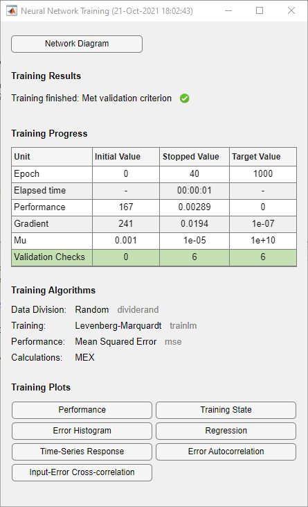
This training stopped when the validation error increased consecutively for six iterations.
Test Network
Test the network. After the network has been trained, you can use it to compute the
network outputs. The following code calculates the network outputs, errors, and overall
performance. Note that to simulate a network with tapped delay lines, you need to assign
the initial values for these delayed signals. This is done with the input states
(xi) and the layer states (ai) provided by
preparets at an earlier
stage.
y = net(x,xi,ai);
e = gsubtract(t,y);
performance = perform(net,t,y)
performance =

    0.0042
View Network
View the network diagram.
view(net)
Analyze Results
Plot the performance training record to check for potential overfitting.
figure, plotperform(tr)
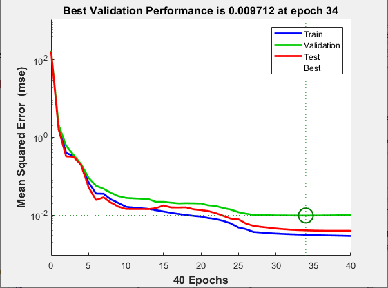
This figure shows that training and validation errors decrease until the highlighted epoch. It does not appear that any overfitting has occurred, because the validation error does not increase before this epoch.
All of the training is done in open loop (also called series-parallel architecture),
including the validation and testing steps. The typical workflow is to fully create the
network in open loop, and only when it has been trained (which includes validation and
testing steps) it is transformed to closed loop for multistep-ahead prediction. Likewise,
the R values in the Neural Net Times Series app are computed
based on the open-loop training results.
Closed Loop Network
Close the loop on the NARX network. When the feedback loop is open on the NARX network, it is performing a one-step-ahead prediction. It is predicting the next value of y(t) from previous values of y(t) and x(t). With the feedback loop closed, it can be used to perform multi-step-ahead predictions. This is because predictions of y(t) will be used in place of actual future values of y(t). The following commands can be used to close the loop and calculate closed-loop performance
netc = closeloop(net);
netc.name = [net.name ' - Closed Loop'];
view(netc)
[xc,xic,aic,tc] = preparets(netc,X,{},T);
yc = netc(xc,xic,aic);
closedLoopPerformance = perform(net,tc,yc)
closedLoopPerformance =
0.4014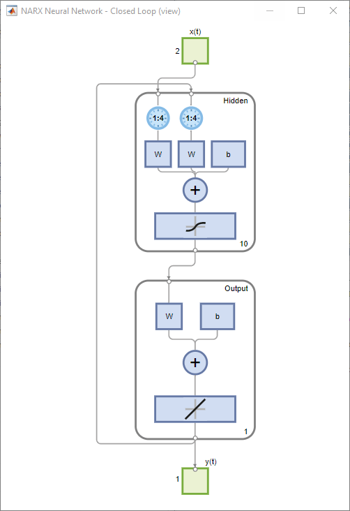
Step-Ahead Prediction Network
Remove a delay from the network, to get the prediction one time step early.
nets = removedelay(net);
nets.name = [net.name ' - Predict One Step Ahead'];
view(nets)
[xs,xis,ais,ts] = preparets(nets,X,{},T);
ys = nets(xs,xis,ais);
stepAheadPerformance = perform(nets,ts,ys)
stepAheadPerformance =
0.0042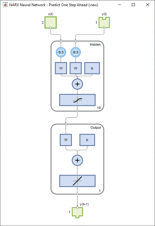
From this figure, you can see that the network is identical to the previous open-loop network, except that one delay has been removed from each of the tapped delay lines. The output of the network is then y(t + 1) instead of y(t). This may sometimes be helpful when a network is deployed for certain applications.
Next Steps
If the network performance is not satisfactory, you could try any of these approaches:
Reset the initial network weights and biases to new values with
initand train again.Increase the number of hidden neurons or the number of delays.
Use a larger training data set.
Increase the number of input values, if more relevant information is available.
Try a different training algorithm (see Training Algorithms).
To get more experience in command-line operations, try some of these tasks:
During training, open a plot window (such as the error correlation plot), and watch it animate.
Plot from the command line with functions such as
plotresponse,ploterrcorrandplotperform.
Each time a neural network is trained can result in a different solution due to random initial weight and bias values and different divisions of data into training, validation, and test sets. As a result, different neural networks trained on the same problem can give different outputs for the same input. To ensure that a neural network of good accuracy has been found, retrain several times.
There are several other techniques for improving upon initial solutions if higher accuracy is desired. For more information, see Improve Shallow Neural Network Generalization and Avoid Overfitting.
See Also
Neural
Net Fitting | Neural
Net Time Series | Neural
Net Pattern Recognition | Neural
Net Clustering | train | preparets | narxnet | closeloop | perform | removedelay
