Texture Classification with Wavelet Image Scattering
This example shows how to classify textures using wavelet image scattering. In addition to Wavelet Toolbox™, this example also requires Parallel Computing Toolbox™ and Image Processing Toolbox™.
In a digital image, texture provides information about the spatial arrangement of color or pixel intensities. Particular spatial arrangements of color or pixel intensities correspond to different appearances and consistencies of the physical material being imaged. Texture classification and segmentation of images has a number of important application areas. A particularly important example is biomedical image analysis where normal and pathologic states are often characterized by morphological and histological characteristics which manifest as differences in texture [4].
Wavelet Image Scattering
For classification problems, it is often useful to map the data into some alternative representation which discards irrelevant information while retaining the discriminative properties of each class. Wavelet image scattering constructs low-variance representations of images which are insensitive to translations and small deformations. Because translations and small deformations in the image do not affect class membership, scattering transform coefficients provide features from which you can build robust classification models.
Wavelet scattering works by cascading the image through a series of wavelet transforms, nonlinearities, and averaging [1][3][5]. The result of this deep feature extraction is that images in the same class are moved closer to each other in the scattering transform representation, while images belonging to different classes are moved farther apart.
KTH-TIPS
This example uses a publicly available texture database, the KTH-TIPS (Textures under varying Illumination, Pose, and Scale) image database [6]. The KTH-TIPS dataset used in this example is the grayscale version. There are 810 images in total with 10 textures and 81 images per texture. The majority of images are 200-by-200 in size. This example assumes you have downloaded the KTH-TIPS grayscale dataset and untarred it so that the 10 texture classes are contained in separate subfolders of a common folder. Each subfolder is named for the class of textures it contains. Untarring the downloaded kth_tips_grey_200x200.tar file is sufficient to provide a top-level folder KTH_TIPS and the required subfolder structure.
Use the imageDatastore to read the data. Set the location property of the imageDatastore to the folder containing the KTH-TIPS database that you have access to.
location = fullfile(tempdir,'kth_tips_grey_200x200','KTH_TIPS');
Imds = imageDatastore(location,'IncludeSubFolders',true,'FileExtensions','.png','LabelSource','foldernames');
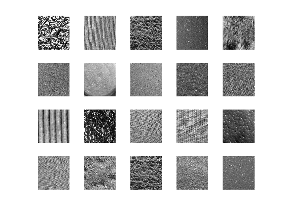
Randomly select and visualize 20 images from the dataset.
numImages = 810;
perm = randperm(numImages,20);
for np = 1:20
    subplot(4,5,np)
    im = imread(Imds.Files{perm(np)});
    imagesc(im);
    colormap gray; axis off;
end

Texture Classification
This example uses MATLAB®'s parallel processing capability through the tall array interface. Start the parallel pool if one is not currently running.
if isempty(gcp)
    parpool;
end
Starting parallel pool (parpool) using the 'local' profile ...
Connected to the parallel pool (number of workers: 6).
For reproducibility, set the random number generator. Shuffle the files of the KTH-TIPS dataset and split the 810 images into two randomly selected sets, one for training and one held-out set for testing. Use approximately 80% of the images for building a predictive model from the scattering transform and use the remainder for testing the model.
rng(100)
Imds = imageDatastore(location,'IncludeSubFolders',true,'FileExtensions','.png','LabelSource','foldernames');
Imds = shuffle(Imds);
[trainImds,testImds] = splitEachLabel(Imds,0.8);
We now have two datasets. The training set consists of 650 images, with 65 images per texture. The testing set consists of 160 images, with 16 images per texture. To verify, count the labels in each dataset.
countEachLabel(trainImds)
ans=10×2 table
        Label         Count
    ______________    _____

    aluminium_foil     65
    brown_bread        65
    corduroy           65
    cotton             65
    cracker            65
    linen              65
    orange_peel        65
    sandpaper          65
    sponge             65
    styrofoam          65
countEachLabel(testImds)
ans=10×2 table
        Label         Count
    ______________    _____

    aluminium_foil     16
    brown_bread        16
    corduroy           16
    cotton             16
    cracker            16
    linen              16
    orange_peel        16
    sandpaper          16
    sponge             16
    styrofoam          16
Create tall arrays for the resized images.
Ttrain = tall(trainImds);
Ttest = tall(testImds);
Create a scattering framework for an image input size of 200-by-200 with an InvarianceScale of 150. The invariance scale hyperparameter is the only one we set in this example. For the other hyperparameters of the scattering transform, use the default values.
sn = waveletScattering2('ImageSize',[200 200],'InvarianceScale',150);
To extract features for classification for each the training and test sets, use the helperScatImages_mean function. The code for helperScatImages_mean is at the end of this example. helperScatImages_mean resizes the images to a common 200-by-200 size and uses the scattering framework, sn, to obtain the feature matrix. In this case, each feature matrix is 391-by-7-by-7. There are 391 scattering paths and each scattering coefficient image is 7-by-7. Finally, helperScatImages_mean obtains the mean along the 2nd and 3rd dimensions to obtain a 391 element feature vector for each image. This is a significant reduction in data from 40,000 elements down to 391.
trainfeatures = cellfun(@(x)helperScatImages_mean(sn,x),Ttrain,'Uni',0);
testfeatures = cellfun(@(x)helperScatImages_mean(sn,x),Ttest,'Uni',0);
Using tall's gather capability, gather all the training and test feature vectors and concatenate them into matrices.
Trainf = gather(trainfeatures);
Evaluating tall expression using the Parallel Pool 'local':
- Pass 1 of 1: Completed in 1 min 39 sec
Evaluation completed in 1 min 39 sec
trainfeatures = cat(2,Trainf{:});
Testf = gather(testfeatures);
Evaluating tall expression using the Parallel Pool 'local': - Pass 1 of 1: Completed in 23 sec Evaluation completed in 23 sec
testfeatures = cat(2,Testf{:});The previous code results in two matrices with row dimensions 391 and column dimension equal to the number of images in the training and test sets, respectively. So each column is a feature vector.
PCA Model and Prediction
This example constructs a simple classifier based on the principal components of the scattering feature vectors for each class. The classifier is implemented in the functions helperPCAModel and helperPCAClassifier. The function helperPCAModel determines the principal components for each digit class based on the scattering features. The code for helperPCAModel is at the end of this example. The function helperPCAClassifier classifies the held-out test data by finding the closest match (best projection) between the principal components of each test feature vector with the training set and assigning the class accordingly. The code for helperPCAClassifier is at the end of this example.
model = helperPCAModel(trainfeatures,30,trainImds.Labels);
predlabels = helperPCAClassifier(testfeatures,model);
After constructing the model and classifying the test set, determine the accuracy of the test set classification.
accuracy = sum(testImds.Labels == predlabels)./numel(testImds.Labels)*100
accuracy = 99.3750
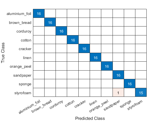
We have achieved 99.375% correct classification, or a 0.625% error rate for the 160 images in the test set. A plot of the confusion matrix shows that our simple model misclassified one texture.
figure
confusionchart(testImds.Labels,predlabels)

Summary
In this example, we used wavelet image scattering to create low-variance representations of textures for classification. Using the scattering transform and a simple principal components classifier, we achieved 99.375% correct classification on a held-out test set. This result is comparable to state-of-the-art performance on the KTH-TIPS database.[2]
References
[1] Bruna, J., and S. Mallat. "Invariant Scattering Convolution Networks." IEEE Transactions on Pattern Analysis and Machine Intelligence. Vol. 35, Number 8, 2013, pp. 1872–1886.
[2] Hayman, E., B. Caputo, M. Fritz, and J. O. Eklundh. “On the Significance of Real-World Conditions for Material Classification.” In Computer Vision - ECCV 2004, edited by Tomás Pajdla and Jiří Matas, 3024:253–66. Berlin, Heidelberg: Springer Berlin Heidelberg, 2004. https://doi.org/10.1007/978-3-540-24673-2_21.
[3] Mallat, S. "Group Invariant Scattering." Communications in Pure and Applied Mathematics. Vol. 65, Number 10, 2012, pp. 1331–1398.
[4] Pujol, O., and P. Radeva. “Supervised Texture Classification for Intravascular Tissue Characterization.” In Handbook of Biomedical Image Analysis, edited by Jasjit S. Suri, David L. Wilson, and Swamy Laxminarayan, 57–109. Boston, MA: Springer US, 2005. https://doi.org/10.1007/0-306-48606-7_2.
[5] Sifre, L., and S. Mallat. "Rotation, scaling and deformation invariant scattering for texture discrimination." 2013 IEEE Conference on Computer Vision and Pattern Recognition. 2013, pp 1233–1240. 10.1109/CVPR.2013.163.
[6] KTH-TIPS image databases homepage. https://www.csc.kth.se/cvap/databases/kth-tips/
Appendix — Supporting Functions
helperScatImages_mean
function features = helperScatImages_mean(sf,x)
x = imresize(x,[200 200]);
smat = featureMatrix(sf,x);
features = mean(mean(smat,2),3);
end
helperPCAModel
function model = helperPCAModel(features,M,Labels)
% This function is only to support wavelet image scattering examples in
% Wavelet Toolbox. It may change or be removed in a future release.
% model = helperPCAModel(features,M,Labels)

% Copyright 2018 bat365

% Initialize structure array to hold the affine model
model = struct('Dim',[],'mu',[],'U',[],'Labels',categorical([]),'s',[]);
model.Dim = M;
% Obtain the number of classes
LabelCategories = categories(Labels);
Nclasses = numel(categories(Labels));
for kk = 1:Nclasses
    Class = LabelCategories{kk};
    % Find indices corresponding to each class
    idxClass = Labels == Class;
    % Extract feature vectors for each class
    tmpFeatures = features(:,idxClass);
    % Determine the mean for each class
    model.mu{kk} = mean(tmpFeatures,2);
    [model.U{kk},model.S{kk}] = scatPCA(tmpFeatures);
    if size(model.U{kk},2) > M
        model.U{kk} = model.U{kk}(:,1:M);
        model.S{kk} = model.S{kk}(1:M);

    end
    model.Labels(kk) = Class;
end

function [u,s,v] = scatPCA(x,M)
	% Calculate the principal components of x along the second dimension.

	if nargin > 1 && M > 0
		% If M is non-zero, calculate the first M principal components.
	    [u,s,v] = svds(x-sig_mean(x),M);
	    s = abs(diag(s)/sqrt(size(x,2)-1)).^2;
	else
		% Otherwise, calculate all the principal components.
        % Each row is an observation, i.e. the number of scattering paths
        % Each column is a class observation
		[u,d] = eig(cov(x'));
		[s,ind] = sort(diag(d),'descend');
		u = u(:,ind);
	end
end
end
helperPCAClassifier
function labels = helperPCAClassifier(features,model)
% This function is only to support wavelet image scattering examples in
% Wavelet Toolbox. It may change or be removed in a future release.
% model is a structure array with fields, M, mu, v, and Labels
% features is the matrix of test data which is Ns-by-L, Ns is the number of
% scattering paths and L is the number of test examples. Each column of
% features is a test example.

% Copyright 2018 bat365

labelIdx = determineClass(features,model);
labels = model.Labels(labelIdx);
% Returns as column vector to agree with imageDatastore Labels
labels = labels(:);


%--------------------------------------------------------------------------
function labelIdx = determineClass(features,model)
% Determine number of classes
Nclasses = numel(model.Labels);
% Initialize error matrix
errMatrix = Inf(Nclasses,size(features,2));
for nc = 1:Nclasses
    % class centroid
    mu = model.mu{nc};
    u = model.U{nc};
    % 1-by-L
    errMatrix(nc,:) = projectionError(features,mu,u);
end
% Determine minimum along class dimension
[~,labelIdx] = min(errMatrix,[],1);


%--------------------------------------------------------------------------
function totalerr = projectionError(features,mu,u)
    %
    Npc = size(u,2);
    L = size(features,2);
    % Subtract class mean: Ns-by-L minus Ns-by-1
    s = features-mu;
    % 1-by-L
    normSqX = sum(abs(s).^2,1)';
    err = Inf(Npc+1,L);
	err(1,:) = normSqX;
    err(2:end,:) = -abs(u'*s).^2;
    % 1-by-L
    totalerr = sqrt(sum(err,1));
end
end
end
