Testing a Normal Mean with Known Standard Deviation, One-Sided

Just to introduce some concepts, let's consider an unrealistically simple example where we want to test a mean and we know the standard deviation. Our data are continuous, and can be modeled with the normal distribution. We need to determine a sample size N so that we can distinguish between a mean of 100 and a mean of 110. We know the standard deviation is 20.

When we carry out a statistical test, we generally test a null hypothesis against an alternative hypothesis. We find a test statistic T, and look at its distribution under the null hypothesis. If we observe an unusual value, say one that has less than 5% chance of happening if the null hypothesis is true, then we reject the null hypothesis in favor of the alternative. (The 5% probability is known as the significance level of the test.) If the value is not unusual, we do not reject the null hypothesis.

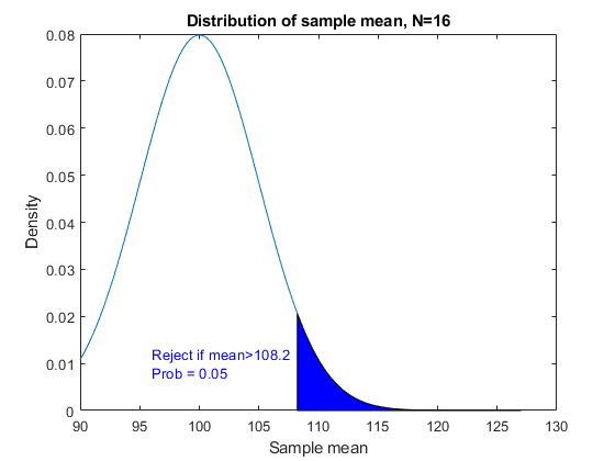
In this case the test statistic T is the sample mean. Under the null hypothesis it has a mean of 100 and a standard deviation of 20/sqrt(N). First let's look at a fixed sample size, say N=16. We will reject the null hypothesis if T is in the shaded region, which is the upper tail of its distribution. That makes this a one-sided test, since we will not reject if T is in the lower tail. The cutoff for this shaded region is 1.6 standard deviations above the mean.

rng(0,'twister');
mu0 = 100;
sig = 20;
N = 16;
alpha = 0.05;
conf = 1-alpha;
cutoff = norminv(conf, mu0, sig/sqrt(N));
x = [linspace(90,cutoff), linspace(cutoff,127)];
y = normpdf(x,mu0,sig/sqrt(N));
h1 = plot(x,y);
xhi = [cutoff, x(x>=cutoff)];
yhi = [0, y(x>=cutoff)];
patch(xhi,yhi,'b');
title('Distribution of sample mean, N=16');
xlabel('Sample mean');
ylabel('Density');
text(96,.01,sprintf('Reject if mean>%.4g\nProb = 0.05',cutoff),'Color','b');

This is how T behaves under the null hypothesis, but what about under an alternative? Our alternative distribution has a mean of 110, as represented by the red curve.

mu1 = 110;
y2 = normpdf(x,mu1,sig/sqrt(N));
h2 = line(x,y2,'Color','r');
yhi = [0, y2(x>=cutoff)];
patch(xhi,yhi,'r','FaceAlpha',0.25);
P = 1 - normcdf(cutoff,mu1,sig/sqrt(N));
text(115,.06,sprintf('Reject if T>%.4g\nProb = %.2g',cutoff,P),'Color',[1 0 0]);
legend([h1 h2],'Null hypothesis','Alternative hypothesis');

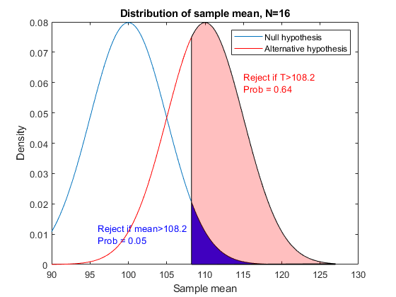
There is a larger chance of rejecting the null hypothesis if the alternative is true. This is just what we want. It's easier to visualize if we look at the cumulative distribution function (cdf) instead of the density (pdf). We can read probabilities directly from this graph, instead of having to compute areas.

ynull = normcdf(x,mu0,sig/sqrt(N));
yalt = normcdf(x,mu1,sig/sqrt(N));
h12 = plot(x,ynull,'b-',x,yalt,'r-');
zval = norminv(conf);
cutoff = mu0 + zval * sig / sqrt(N);
line([90,cutoff,cutoff],[conf, conf, 0],'LineStyle',':');
msg = sprintf(' Cutoff = 100 + %.2g \\times 20 / \\surd{n}',zval);
text(cutoff,.15,msg,'Color','b');
text(min(x),conf,sprintf('   %g%% test',100*alpha),'Color','b',...
                         'verticalalignment','top')
palt = normcdf(cutoff,mu1,sig/sqrt(N));
line([90,cutoff],[palt,palt],'Color','r','LineStyle',':');
text(91,palt+.02,sprintf(' Power is 1-%.2g = %.2g',palt,1-palt),'Color',[1 0 0]);
legend(h12,'Null hypothesis','Alternative hypothesis');

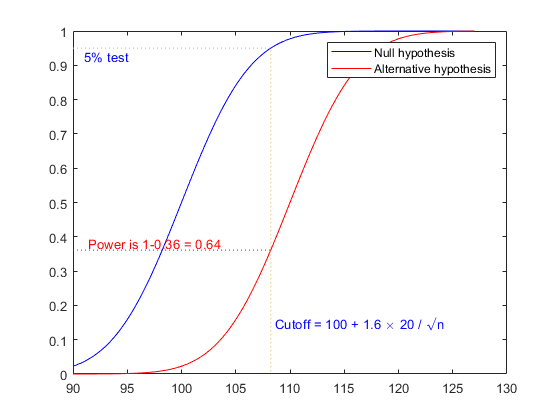
This graph shows the probability of getting a significant statistic (rejecting the null hypothesis) for two different mu values when N=16.

The power function is defined as the probability of rejecting the null hypothesis when the alternative is true. It depends on the value of the alternative and on the sample size. We'll graph the power (which is one minus the cdf) as a function of N, fixing the alternative at 110. We'll select N to achieve a power of 80%. The graph shows that we need about N=25.

DesiredPower = 0.80;
Nvec = 1:30;
cutoff = mu0 + norminv(conf)*sig./sqrt(Nvec);
power = 1 - normcdf(cutoff, mu1, sig./sqrt(Nvec));
plot(Nvec,power,'bo-',[0 30],[DesiredPower DesiredPower],'k:');
xlabel('N = sample size')
ylabel('Power')
title('Power function for the alternative: \mu = 110')

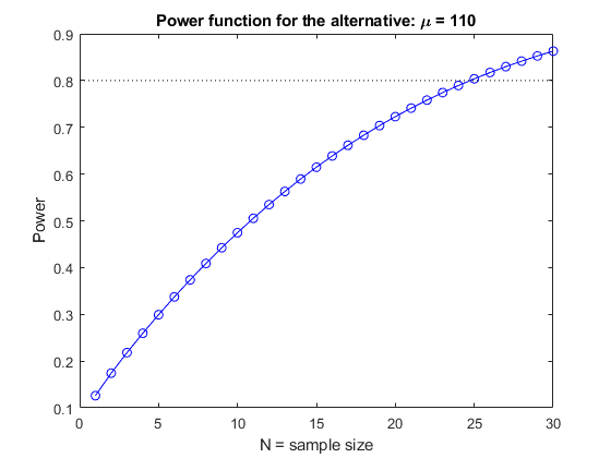
In this overly simple example there is a formula to compute the required value directly to get a power of 80%:

mudiff = (mu1 - mu0) / sig;
N80 = ceil(((norminv(1-DesiredPower)-norminv(conf)) / mudiff)^2)

N80 =

    25

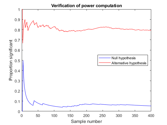
To verify that this works, let's do a Monte Carlo simulation and generate 400 samples of size 25 both under the null hypothesis with mean 100, and under the alternative hypothesis with mean 110. If we test each sample to see if its mean is 100, we should expect about 5% of the first group and 80% of the second group to be significant.

nsamples = 400;
samplenum = 1:nsamples;
N = 25;
h0 = zeros(1,nsamples);
h1 = h0;
for j = 1:nsamples
    Z0 = normrnd(mu0,sig,N,1);
    h0(j) = ztest(Z0,mu0,sig,alpha,'right');
    Z1 = normrnd(mu1,sig,N,1);
    h1(j) = ztest(Z1,mu0,sig,alpha,'right');
end
p0 = cumsum(h0) ./ samplenum;
p1 = cumsum(h1) ./ samplenum;
plot(samplenum,p0,'b-',samplenum,p1,'r-')
xlabel('Sample number')
ylabel('Proportion significant')
title('Verification of power computation')
legend('Null hypothesis','Alternative hypothesis','Location','East')

Testing a Normal Mean with Unknown Standard Deviation, Two-Sided

Now let's suppose we don't know the standard deviation, and we want to perform a two-sided test, that is, one that rejects the null hypothesis whether the sample mean is too high or too low.

The test statistic is a t statistic, which is the difference between the sample mean and the mean being tested, divided by the standard error of the mean. Under the null hypothesis, this has Student's t distribution with N-1 degrees of freedom. Under the alternative hypothesis, the distribution is a noncentral t distribution with a noncentrality parameter equal to the normalized difference between the true mean and the mean being tested.

For this two-sided test we have to allocate the 5% chance of an error under the null hypothesis equally to both tails, and reject if the test statistic is too extreme in either direction. We also have to consider both tails under any alternative.

N = 16;
df = N-1;
alpha = 0.05;
conf = 1-alpha;
cutoff1 = tinv(alpha/2,df);
cutoff2 = tinv(1-alpha/2,df);
x = [linspace(-5,cutoff1), linspace(cutoff1,cutoff2),linspace(cutoff2,5)];
y = tpdf(x,df);
h1 = plot(x,y);
xlo = [x(x<=cutoff1),cutoff1];
ylo = [y(x<=cutoff1),0];
xhi = [cutoff2,x(x>=cutoff2)];
yhi = [0, y(x>=cutoff2)];
patch(xlo,ylo,'b');
patch(xhi,yhi,'b');
title('Distribution of t statistic, N=16');
xlabel('t');
ylabel('Density');
text(2.5,.05,sprintf('Reject if t>%.4g\nProb = 0.025',cutoff2),'Color','b');
text(-4.5,.05,sprintf('Reject if t<%.4g\nProb = 0.025',cutoff1),'Color','b');

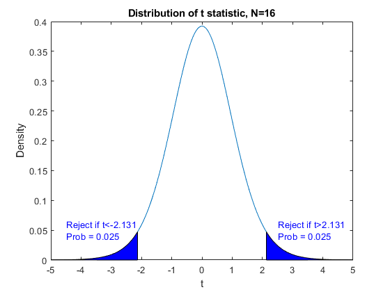
Instead of examining the power function just under the null hypothesis and a single alternative value of mu, we can look at it as a function of mu. The power increases as mu moves away from the null hypothesis value in either direction. We can use the sampsizepwr function to compute the power. For a power calculation we need to specify a value for the standard deviation, which we suspect will be roughly 20. Here's a picture of the power function for a sample size N=16.

N = 16;
x = linspace(90,127);
power = sampsizepwr('t',[100 20],x,[],N);
plot(x,power);
xlabel('True mean')
ylabel('Power')
title('Power function for N=16')

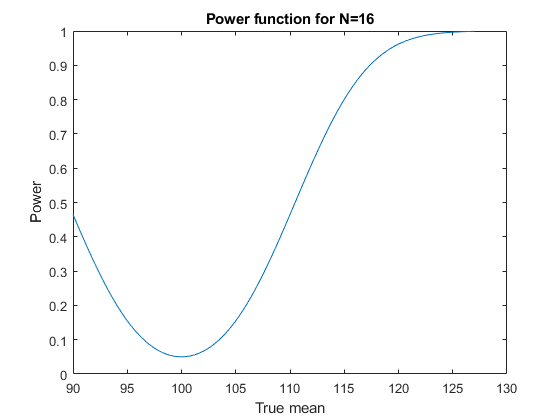
We want a power of 80% when the mean is 110. According to this graph, our power is less than 50% with a sample size of N=16. What sample size will give the power we want?

N = sampsizepwr('t',[100 20],110,0.8)

N =

    34

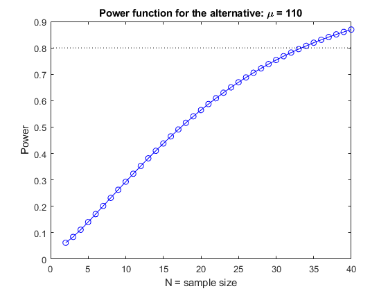
We need a sample size of about 34. Compared with the previous example, we need to take nine additional observations to allow a two-sided test and to make up for not knowing the true standard deviation.

We can make a plot of the power function for various values of N.

Nvec = 2:40;
power = sampsizepwr('t',[100 20],110,[],Nvec);
plot(Nvec,power,'bo-',[0 40],[DesiredPower DesiredPower],'k:');
xlabel('N = sample size')
ylabel('Power')
title('Power function for the alternative: \mu = 110')

And we can do a simulation similar to the earlier one to verify that we get the power we need.

nsamples = 400;
samplenum = 1:nsamples;
N = 34;
h0 = zeros(1,nsamples);
h1 = h0;
for j = 1:nsamples
    Z0 = normrnd(mu0,sig,N,1);
    h0(j) = ttest(Z0,mu0,alpha);
    Z1 = normrnd(mu1,sig,N,1);
    h1(j) = ttest(Z1,mu0,alpha);
end
p0 = cumsum(h0) ./ samplenum;
p1 = cumsum(h1) ./ samplenum;
plot(samplenum,p0,'b-',samplenum,p1,'r-')
xlabel('Sample number')
ylabel('Proportion significant')
title('Verification of power computation')
legend('Null hypothesis','Alternative hypothesis','Location','East')

Suppose we could afford to take a sample size of 50. Presumably our power for detecting the alternative value mu=110 would be larger than 80%. If we maintain the power at 80%, what alternative could we detect?

mu1 = sampsizepwr('t',[100 20],[],.8,50)

mu1 =

  108.0837

Testing a Proportion

Now let's turn to the problem of determining the sample size needed to distinguish between two proportions. Suppose that we are sampling a population in which about 30% favor some candidate, and we want to sample enough people so we can distinguish this value from 33%.

The idea here is the same as before. Here we can use the sample count as our test statistic. This count has a binomial distribution. For any sample size N we can compute the cutoff for rejecting the null hypothesis P=0.30. For N=100, for instance, we would reject the null hypothesis if the sample count is larger than a cutoff value computed as follows:

N = 100;
alpha = 0.05;
p0 = 0.30;
p1 = 0.33;
cutoff = binoinv(1-alpha, N, p0)

cutoff =

    38

A complication with the binomial distribution comes because it is discrete. The probability of exceeding the cutoff value is not exactly 5%:

1 - binocdf(cutoff, N, p0)

ans =

    0.0340

Once again, let's compute the power against the alternative P=0.33 for a range of sample sizes. We'll use a one-sided (right-tailed) test because we're interested only in alternative values greater than 30%.

Nvec = 50:50:2000;
power = sampsizepwr('p',p0,p1,[],Nvec,'tail','right');
plot(Nvec,power,'bo-',[0 2000],[DesiredPower DesiredPower],'k:');
xlabel('N = sample size')
ylabel('Power')
title('Power function for the alternative: p = 0.33')

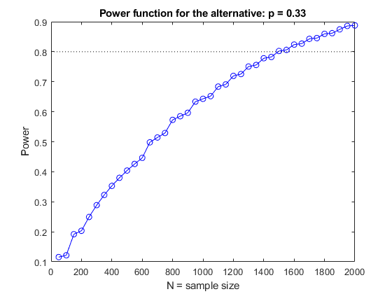
We can use the sampsizepwr function to request the sample size required for a power of 80%.

approxN = sampsizepwr('p',p0,p1,0.80,[],'tail','right')

Warning: Values N>200 are approximate.  Plotting the power as a function
of N may reveal lower N values that have the required power. 

approxN =

        1500

A warning message informs us that the answer is just approximate. If we look at the power function for different sample sizes, we can see that the function is generally increasing, but irregular because the binomial distribution is discrete. Let's look at the probability of rejecting the null hypothesis for both p=0.30 and p=0.33 in the range of samples sizes from 1470 to 1480.

subplot(3,1,1);
Nvec = 1470:1480;
power = sampsizepwr('p',p0,p1,[],Nvec,'tail','right');
plot(Nvec,power,'ro-',[min(Nvec),max(Nvec)],[DesiredPower DesiredPower],'k:');
ylabel(sprintf('Prob[T>cutoff]\nif p=0.33'))
h_gca = gca;
h_gca.XTickLabel = '';
ylim([.78, .82]);

subplot(3,1,2);
alf = sampsizepwr('p',p0,p0,[],Nvec,'tail','right');
plot(Nvec,alf,'bo-',[min(Nvec),max(Nvec)],[alpha alpha],'k:');
ylabel(sprintf('Prob[T>cutoff]\nif p=0.30'))
h_gca = gca;
h_gca.XTickLabel = '';
ylim([.04, .06]);

subplot(3,1,3);
cutoff = binoinv(1-alpha, Nvec, p0);
plot(Nvec,cutoff,'go-');
xlabel('N = sample size')
ylabel('Cutoff')

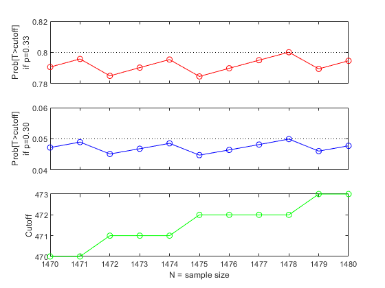
This plot reveals that the power function curve (top plot) is not only irregular, but also decreases at some sample sizes. These are the sample sizes for which it is necessary to increase the cutoff value (bottom plot) in order to keep the significance level (middle plot) no larger than 5%. We can find a smaller sample size within this range that gives the desired power of 80%:

min(Nvec(power>=0.80))

ans =

        1478

Testing a Correlation

In the examples we've considered so far, we were able to figure out the cutoff for a test statistic to achieve a certain significance level, and to calculate the probability of exceeding that cutoff under an alternative hypothesis. For our final example, let's consider a problem where that is not so easy.

Imagine we can take samples from two variables X and Y, and we want to know what sample size we would need to test whether they are uncorrelated versus the alternative that their correlation is as high as 0.4. Although it is possible to work out the distribution of the sample correlation by transforming it to a t distribution, let's use a method that we can use even in problems where we can't work out the distribution of the test statistic.

For a given sample size, we can use Monte Carlo simulation to determine an approximate cutoff value for a test of the correlation. Let's do a large simulation run so we can get this value accurately. We'll start with a sample size of 25.

nsamples = 10000;
N = 25;
alpha = 0.05;
conf = 1-alpha;
r = zeros(1,nsamples);
for j = 1:nsamples
    xy = normrnd(0,1,N,2);
    r(j) = corr(xy(:,1),xy(:,2));
end
cutoff = quantile(r,conf)

cutoff =

    0.3372

Then we can generate samples under the alternative hypothesis, and estimate the power of the test.

nsamples = 1000;
mu = [0; 0];
sig = [1 0.4; 0.4 1];
r = zeros(1,nsamples);
for j = 1:nsamples
    xy = mvnrnd(mu,sig,N);
    r(j) = corr(xy(:,1),xy(:,2));
end
[power,powerci] = binofit(sum(r>cutoff),nsamples)

power =

    0.6470


powerci =

    0.6165    0.6767

We estimate the power to be 65%, and we have 95% confidence that the true value is between 62% and 68%. To get a power of 80%, we need a larger sample size. We might try increasing N to 50, estimating the cutoff value for this sample size, and repeating the power simulation.

nsamples = 10000;
N = 50;
alpha = 0.05;
conf = 1-alpha;
r = zeros(1,nsamples);
for j = 1:nsamples
    xy = normrnd(0,1,N,2);
    r(j) = corr(xy(:,1),xy(:,2));
end
cutoff = quantile(r,conf)

nsamples = 1000;
mu = [0; 0];
sig = [1 0.4; 0.4 1];
r = zeros(1,nsamples);
for j = 1:nsamples
    xy = mvnrnd(mu,sig,N);
    r(j) = corr(xy(:,1),xy(:,2));
end
[power,powerci] = binofit(sum(r>cutoff),nsamples)

cutoff =

    0.2315


power =

    0.8990


powerci =

    0.8786    0.9170

This sample size gives a power better than our target of 80%. We could continue experimenting this way, trying to find a sample size less than 50 that would meet our requirements.

Conclusion

The probability functions in the Statistics and Machine Learning Toolbox can be used to determine the sample size required to achieve a desired level of power in a hypothesis test. In some problems the sample size can be compute directly; in others it is necessary to search over a range of sample sizes until the right value is found. Random number generators can help verify that the desired power is met, and can also be used to study the power of a specific test under alternative conditions.