Obtain the data

Import the data into your workspace. Extract the last data column into a variable named Y.

gunzip('https://archive.ics.uci.edu/ml/machine-learning-databases/covtype/covtype.data.gz')
load covtype.data
Y = covtype(:,end);
covtype(:,end) = [];

Examine the response data

tabulate(Y)

  Value    Count   Percent
      1    211840     36.46%
      2    283301     48.76%
      3    35754      6.15%
      4     2747      0.47%
      5     9493      1.63%
      6    17367      2.99%
      7    20510      3.53%

There are hundreds of thousands of data points. Those of class 4 are less than 0.5% of the total. This imbalance indicates that RUSBoost is an appropriate algorithm.

Partition the data for quality assessment

Use half the data to fit a classifier, and half to examine the quality of the resulting classifier.

rng(10,'twister')         % For reproducibility
part = cvpartition(Y,'Holdout',0.5);
istrain = training(part); % Data for fitting
istest = test(part);      % Data for quality assessment
tabulate(Y(istrain))

  Value    Count   Percent
      1    105919     36.46%
      2    141651     48.76%
      3    17877      6.15%
      4     1374      0.47%
      5     4747      1.63%
      6     8684      2.99%
      7    10254      3.53%

Create the ensemble

Use deep trees for higher ensemble accuracy. To do so, set the trees to have maximal number of decision splits of N, where N is the number of observations in the training sample. Set LearnRate to 0.1 in order to achieve higher accuracy as well. The data is large, and, with deep trees, creating the ensemble is time consuming.

N = sum(istrain);         % Number of observations in the training sample
t = templateTree('MaxNumSplits',N);
tic
rusTree = fitcensemble(covtype(istrain,:),Y(istrain),'Method','RUSBoost', ...
    'NumLearningCycles',1000,'Learners',t,'LearnRate',0.1,'nprint',100);

Training RUSBoost...
Grown weak learners: 100
Grown weak learners: 200
Grown weak learners: 300
Grown weak learners: 400
Grown weak learners: 500
Grown weak learners: 600
Grown weak learners: 700
Grown weak learners: 800
Grown weak learners: 900
Grown weak learners: 1000

toc

Elapsed time is 242.836734 seconds.

Inspect the classification error

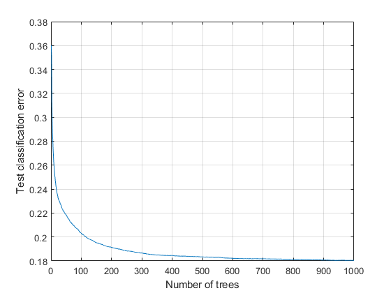
Plot the classification error against the number of members in the ensemble.

figure;
tic
plot(loss(rusTree,covtype(istest,:),Y(istest),'mode','cumulative'));
toc

Elapsed time is 164.470086 seconds.

grid on;
xlabel('Number of trees');
ylabel('Test classification error');

The ensemble achieves a classification error of under 20% using 116 or more trees. For 500 or more trees, the classification error decreases at a slower rate.

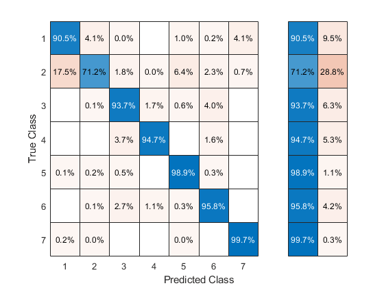
Examine the confusion matrix for each class as a percentage of the true class.

tic
Yfit = predict(rusTree,covtype(istest,:));
toc

Elapsed time is 132.353489 seconds.

confusionchart(Y(istest),Yfit,'Normalization','row-normalized','RowSummary','row-normalized')

All classes except class 2 have over 90% classification accuracy. But class 2 makes up close to half the data, so the overall accuracy is not that high.

Compact the ensemble

The ensemble is large. Remove the data using the compact method.

cmpctRus = compact(rusTree);

sz(1) = whos('rusTree');
sz(2) = whos('cmpctRus');
[sz(1).bytes sz(2).bytes]

ans = 1×2
109 ×

    1.6579    0.9423

The compacted ensemble is about half the size of the original.

Remove half the trees from cmpctRus. This action is likely to have minimal effect on the predictive performance, based on the observation that 500 out of 1000 trees give nearly optimal accuracy.

cmpctRus = removeLearners(cmpctRus,[500:1000]);

sz(3) = whos('cmpctRus');
sz(3).bytes

ans = 452868660

The reduced compact ensemble takes about a quarter of the memory of the full ensemble. Its overall loss rate is under 19%:

L = loss(cmpctRus,covtype(istest,:),Y(istest))

L = 0.1833

The predictive accuracy on new data might differ, because the ensemble accuracy might be biased. The bias arises because the same data used for assessing the ensemble was used for reducing the ensemble size. To obtain an unbiased estimate of requisite ensemble size, you should use cross validation. However, that procedure is time consuming.