Classification Using Nearest Neighbors
Pairwise Distance Metrics
Categorizing query points based on their distance to points in a training data set can be a simple yet effective way of classifying new points. You can use various metrics to determine the distance, described next. Use pdist2 to find the distance between a set of data and query points.
Distance Metrics
Given an mx-by-n data matrix X, which is treated as mx (1-by-n) row vectors x1, x2, ..., xmx, and an my-by-n data matrix Y, which is treated as my (1-by-n) row vectors y1, y2, ...,ymy, the various distances between the vector xs and yt are defined as follows:
Euclidean distance
The Euclidean distance is a special case of the Minkowski distance, where p = 2.
Specify Euclidean distance by setting the
Distanceparameter to'euclidean'.Standardized Euclidean distance
where V is the n-by-n diagonal matrix whose jth diagonal element is (S(j))2, where S is a vector of scaling factors for each dimension.
Specify standardized Euclidean distance by setting the
Distanceparameter to'seuclidean'.Fast Euclidean distance is the same as Euclidean distance, computed by using an alternative algorithm that saves time when the number of predictors is at least 10. In some cases, this faster algorithm can reduce accuracy. Does not support sparse data. See Fast Euclidean Distance Algorithm.
Specify fast Euclidean distance by setting the
Distanceparameter to'fasteuclidean'.Fast standardized Euclidean distance is the same as standardized Euclidean distance, computed by using an alternative algorithm that saves time when the number of predictors is at least 10. In some cases, this faster algorithm can reduce accuracy. Does not support sparse data. See Fast Euclidean Distance Algorithm.
Specify fast standardized Euclidean distance by setting the
Distanceparameter to'fastseuclidean'.Mahalanobis distance
where C is the covariance matrix.
Specify Mahalanobis distance by setting the
Distanceparameter to'mahalanobis'.City block distance
The city block distance is a special case of the Minkowski distance, where p = 1.
Specify city block distance by setting the
Distanceparameter to'cityblock'.Minkowski distance
For the special case of p = 1, the Minkowski distance gives the city block distance. For the special case of p = 2, the Minkowski distance gives the Euclidean distance. For the special case of p = ∞, the Minkowski distance gives the Chebychev distance.
Specify Minkowski distance by setting the
Distanceparameter to'minkowski'.Chebychev distance
The Chebychev distance is a special case of the Minkowski distance, where p = ∞.
Specify Chebychev distance by setting the
Distanceparameter to'chebychev'.Cosine distance
Specify cosine distance by setting the
Distanceparameter to'cosine'.Correlation distance
where
and
Specify correlation distance by setting the
Distanceparameter to'correlation'.Hamming distance is the percentage of coordinates that differ:
Specify Hamming distance by setting the
Distanceparameter to'hamming'.Jaccard distance is one minus the Jaccard coefficient, which is the percentage of nonzero coordinates that differ:
Specify Jaccard distance by setting the
Distanceparameter to'jaccard'.Spearman distance is one minus the sample Spearman's rank correlation between observations (treated as sequences of values):
where
Specify Spearman distance by setting the
Distanceparameter to'spearman'.
k-Nearest Neighbor Search and Radius Search
Given a set X of n points and a distance function, k-nearest neighbor (kNN) search lets you find the k closest points in X to a query point or set of points Y. The kNN search technique and kNN-based algorithms are widely used as benchmark learning rules. The relative simplicity of the kNN search technique makes it easy to compare the results from other classification techniques to kNN results. The technique has been used in various areas such as:
bioinformatics
image processing and data compression
document retrieval
computer vision
multimedia database
marketing data analysis
You can use kNN search for other machine learning algorithms, such as:
kNN classification
local weighted regression
missing data imputation and interpolation
density estimation
You can also use kNN search with many distance-based learning functions, such as K-means clustering.
In contrast, for a positive real value r, rangesearch finds all points in X that are within a distance r of each point in Y. This fixed-radius search is closely related to kNN search, as it supports the same distance metrics and search classes, and uses the same search algorithms.
k-Nearest Neighbor Search Using Exhaustive Search
When your input data meets any of the following criteria, knnsearch uses the exhaustive search method by default to find the k-nearest neighbors:
The number of columns of
Xis more than 10.Xis sparse.The distance metric is either:
'seuclidean''mahalanobis''cosine''correlation''spearman''hamming''jaccard'A custom distance function
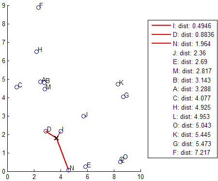
knnsearch also uses the exhaustive search method if your search object is an ExhaustiveSearcher model object. The exhaustive search method finds the distance from each query point to every point in X, ranks them in ascending order, and returns the k points with the smallest distances. For example, this diagram shows the k = 3 nearest neighbors.
k-Nearest Neighbor Search Using a Kd-Tree
When your input data meets all of the following criteria, knnsearch creates a Kd-tree by default to find the k-nearest neighbors:
The number of columns of
Xis less than 10.Xis not sparse.The distance metric is either:
'euclidean'(default)'cityblock''minkowski''chebychev'
knnsearch also uses a Kd-tree if your search object is a KDTreeSearcher model object.
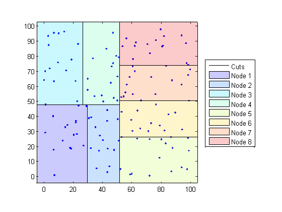
Kd-trees divide your data into nodes with at most BucketSize (default is 50) points per node, based on coordinates (as opposed to categories). The following diagrams illustrate this concept using patch objects to color code the different “buckets.”
When you want to find the k-nearest neighbors to a given query point, knnsearch does the following:
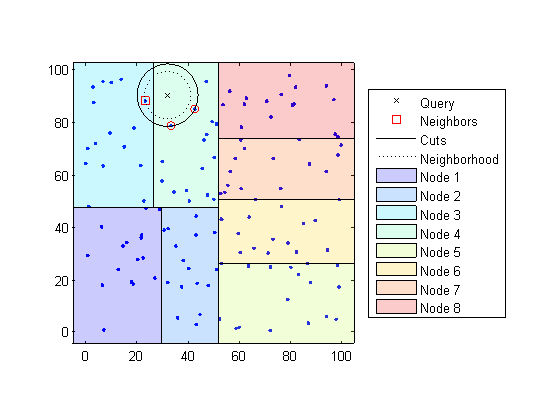
Determines the node to which the query point belongs. In the following example, the query point (32,90) belongs to Node 4.
Finds the closest k points within that node and its distance to the query point. In the following example, the points in red circles are equidistant from the query point, and are the closest points to the query point within Node 4.
Chooses all other nodes having any area that is within the same distance, in any direction, from the query point to the kth closest point. In this example, only Node 3 overlaps the solid black circle centered at the query point with radius equal to the distance to the closest points within Node 4.
Searches nodes within that range for any points closer to the query point. In the following example, the point in a red square is slightly closer to the query point than those within Node 4.
Using a Kd-tree for large data sets with fewer than 10 dimensions (columns) can be much more efficient than using the exhaustive search method, as knnsearch needs to calculate only a subset of the distances. To maximize the efficiency of Kd-trees, use a KDTreeSearcher model.
What Are Search Model Objects?
Basically, model objects are a convenient way of storing information. Related models have the same properties with values and types relevant to a specified search method. In addition to storing information within models, you can perform certain actions on models.
You can efficiently perform a k-nearest neighbors search on your
search model using knnsearch. Or, you can search for all neighbors
within a specified radius using your search model and rangesearch. In addition, there are generic knnsearch and rangesearch functions that search without
creating or using a model.
To determine which type of model and search method is best for your data, consider the following:
Does your data have many columns, say more than 10? The
ExhaustiveSearchermodel may perform better.Is your data sparse? Use the
ExhaustiveSearchermodel.Do you want to use one of these distance metrics to find the nearest neighbors? Use the
ExhaustiveSearchermodel.'seuclidean''mahalanobis''cosine''correlation''spearman''hamming''jaccard'A custom distance function
Is your data set huge (but with fewer than 10 columns)? Use the
KDTreeSearchermodel.Are you searching for the nearest neighbors for a large number of query points? Use the
KDTreeSearchermodel.
Classify Query Data
This example shows how to classify query data by:
Growing a Kd-tree
Conducting a k nearest neighbor search using the grown tree.
Assigning each query point the class with the highest representation among their respective nearest neighbors.
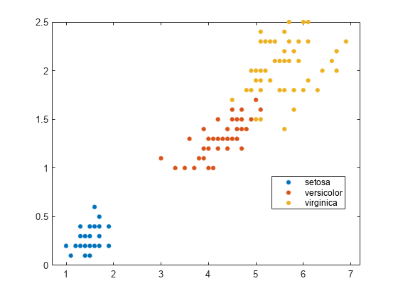
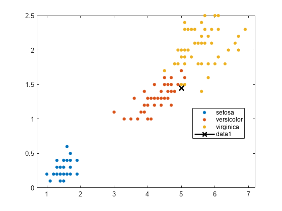
Classify a new point based on the last two columns of the Fisher iris data. Using only the last two columns makes it easier to plot.
load fisheriris
x = meas(:,3:4);
gscatter(x(:,1),x(:,2),species)
legend('Location','best')
Plot the new point.
newpoint = [5 1.45];
line(newpoint(1),newpoint(2),'marker','x','color','k',...
   'markersize',10,'linewidth',2)
Prepare a Kd-tree neighbor searcher model.
Mdl = KDTreeSearcher(x)
Mdl =
  KDTreeSearcher with properties:

       BucketSize: 50
         Distance: 'euclidean'
    DistParameter: []
                X: [150x2 double]
Mdl is a KDTreeSearcher model. By default, the distance metric it uses to search for neighbors is Euclidean distance.
Find the 10 sample points closest to the new point.
[n,d] = knnsearch(Mdl,newpoint,'k',10);
line(x(n,1),x(n,2),'color',[.5 .5 .5],'marker','o',...
    'linestyle','none','markersize',10)
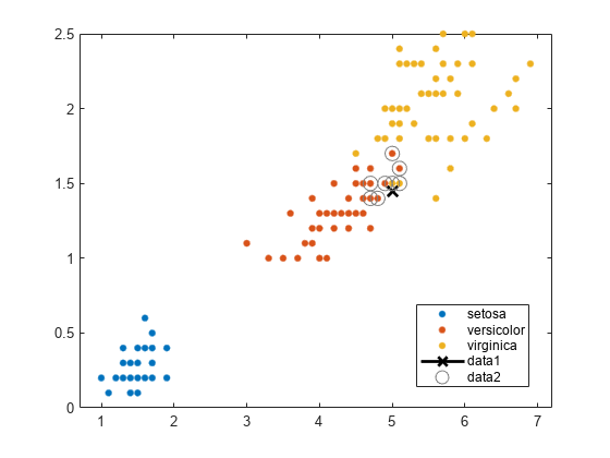
It appears that knnsearch has found only the nearest eight neighbors. In fact, this particular dataset contains duplicate values.
x(n,:)
ans = 10×2

    5.0000    1.5000
    4.9000    1.5000
    4.9000    1.5000
    5.1000    1.5000
    5.1000    1.6000
    4.8000    1.4000
    5.0000    1.7000
    4.7000    1.4000
    4.7000    1.4000
    4.7000    1.5000
Make the axes equal so the calculated distances correspond to the apparent distances on the plot axis equal and zoom in to see the neighbors better.
xlim([4.5 5.5]);
ylim([1 2]);
axis square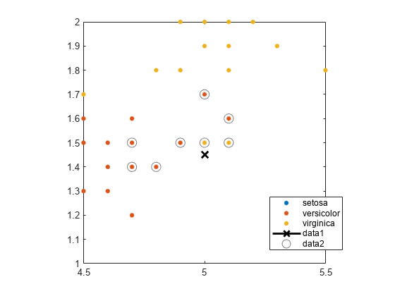
Find the species of the 10 neighbors.
tabulate(species(n))
       Value    Count   Percent
   virginica        2     20.00%
  versicolor        8     80.00%
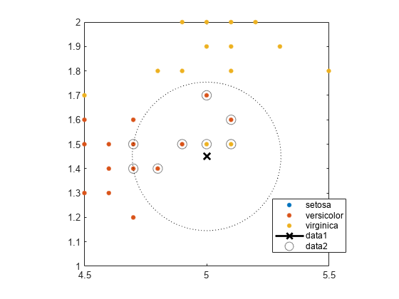
Using a rule based on the majority vote of the 10 nearest neighbors, you can classify this new point as a versicolor.
Visually identify the neighbors by drawing a circle around the group of them. Define the center and diameter of a circle, based on the location of the new point.
ctr = newpoint - d(end);
diameter = 2*d(end);
% Draw a circle around the 10 nearest neighbors.
h = rectangle('position',[ctr,diameter,diameter],...
   'curvature',[1 1]);
h.LineStyle = ':';
Using the same dataset, find the 10 nearest neighbors to three new points.
figure
newpoint2 = [5 1.45;6 2;2.75 .75];
gscatter(x(:,1),x(:,2),species)
legend('location','best')
[n2,d2] = knnsearch(Mdl,newpoint2,'k',10);
line(x(n2,1),x(n2,2),'color',[.5 .5 .5],'marker','o',...
   'linestyle','none','markersize',10)
line(newpoint2(:,1),newpoint2(:,2),'marker','x','color','k',...
   'markersize',10,'linewidth',2,'linestyle','none')
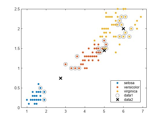
Find the species of the 10 nearest neighbors for each new point.
tabulate(species(n2(1,:)))
       Value    Count   Percent
   virginica        2     20.00%
  versicolor        8     80.00%
tabulate(species(n2(2,:)))
      Value    Count   Percent
  virginica       10    100.00%
tabulate(species(n2(3,:)))
       Value    Count   Percent
  versicolor        7     70.00%
      setosa        3     30.00%
For more examples using knnsearch methods and function, see the individual reference pages.
Find Nearest Neighbors Using a Custom Distance Metric
This example shows how to find the indices of the three nearest observations in X to each observation in Y with respect to the chi-square distance. This distance metric is used in correspondence analysis, particularly in ecological applications.
Randomly generate normally distributed data into two matrices. The number of rows can vary, but the number of columns must be equal. This example uses 2-D data for plotting.
rng(1) % For reproducibility
X = randn(50,2);
Y = randn(4,2);

h = zeros(3,1);
figure
h(1) = plot(X(:,1),X(:,2),'bx');
hold on
h(2) = plot(Y(:,1),Y(:,2),'rs','MarkerSize',10);
title('Heterogeneous Data')
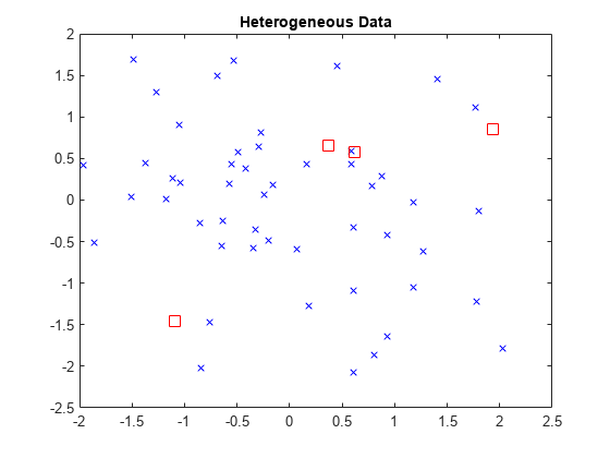
The rows of X and Y correspond to observations, and the columns are, in general, dimensions (for example, predictors).
The chi-square distance between j-dimensional points x and z is
where is the weight associated with dimension j.
Choose weights for each dimension, and specify the chi-square distance function. The distance function must:
Take as input arguments one row of
X, e.g.,x, and the matrixZ.Compare
xto each row ofZ.Return a vector
Dof length , where is the number of rows ofZ. Each element ofDis the distance between the observation corresponding toxand the observations corresponding to each row ofZ.
w = [0.4; 0.6];
chiSqrDist = @(x,Z)sqrt(((x-Z).^2)*w);
This example uses arbitrary weights for illustration.
Find the indices of the three nearest observations in X to each observation in Y.
k = 3;
[Idx,D] = knnsearch(X,Y,'Distance',chiSqrDist,'k',k);
idx and D are 4-by-3 matrices.
idx(j,1)is the row index of the closest observation inXto observation j ofY, andD(j,1)is their distance.idx(j,2)is the row index of the next closest observation inXto observation j ofY, andD(j,2)is their distance.And so on.
Identify the nearest observations in the plot.
for j = 1:k
    h(3) = plot(X(Idx(:,j),1),X(Idx(:,j),2),'ko','MarkerSize',10);
end
legend(h,{'\texttt{X}','\texttt{Y}','Nearest Neighbor'},'Interpreter','latex')
title('Heterogeneous Data and Nearest Neighbors')
hold off
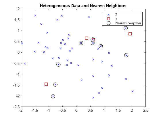
Several observations of Y share nearest neighbors.
Verify that the chi-square distance metric is equivalent to the Euclidean distance metric, but with an optional scaling parameter.
[IdxE,DE] = knnsearch(X,Y,'Distance','seuclidean','k',k, ...
    'Scale',1./(sqrt(w)));
AreDiffIdx = sum(sum(Idx ~= IdxE))
AreDiffIdx = 0
AreDiffDist = sum(sum(abs(D - DE) > eps))
AreDiffDist = 0
The indices and distances between the two implementations of three nearest neighbors are practically equivalent.
K-Nearest Neighbor Classification for Supervised Learning
The ClassificationKNN classification model lets you:
Prepare your data for classification according to the procedure in Steps in Supervised Learning. Then, construct the classifier using fitcknn.
Construct KNN Classifier
This example shows how to construct a k-nearest neighbor classifier for the Fisher iris data.
Load the Fisher iris data.
load fisheriris
X = meas;    % Use all data for fitting
Y = species; % Response data
Construct the classifier using fitcknn.
Mdl = fitcknn(X,Y)
Mdl =
  ClassificationKNN
             ResponseName: 'Y'
    CategoricalPredictors: []
               ClassNames: {'setosa'  'versicolor'  'virginica'}
           ScoreTransform: 'none'
          NumObservations: 150
                 Distance: 'euclidean'
             NumNeighbors: 1
A default k-nearest neighbor classifier uses a single nearest neighbor only. Often, a classifier is more robust with more neighbors than that.
Change the neighborhood size of Mdl to 4, meaning that Mdl classifies using the four nearest neighbors.
Mdl.NumNeighbors = 4;
Examine Quality of KNN Classifier
This example shows how to examine the quality of a k-nearest neighbor classifier using resubstitution and cross validation.
Construct a KNN classifier for the Fisher iris data as in Construct KNN Classifier.
load fisheriris
X = meas;
Y = species;
rng(10); % For reproducibility
Mdl = fitcknn(X,Y,'NumNeighbors',4);
Examine the resubstitution loss, which, by default, is the fraction of misclassifications from the predictions of Mdl. (For nondefault cost, weights, or priors, see loss.)
rloss = resubLoss(Mdl)
rloss = 0.0400
The classifier predicts incorrectly for 4% of the training data.
Construct a cross-validated classifier from the model.
CVMdl = crossval(Mdl);
Examine the cross-validation loss, which is the average loss of each cross-validation model when predicting on data that is not used for training.
kloss = kfoldLoss(CVMdl)
kloss = 0.0333
The cross-validated classification accuracy resembles the resubstitution accuracy. Therefore, you can expect Mdl to misclassify approximately 4% of new data, assuming that the new data has about the same distribution as the training data.
Predict Classification Using KNN Classifier
This example shows how to predict classification for a k-nearest neighbor classifier.
Construct a KNN classifier for the Fisher iris data as in Construct KNN Classifier.
load fisheriris
X = meas;
Y = species;
Mdl = fitcknn(X,Y,'NumNeighbors',4);
Predict the classification of an average flower.
flwr = mean(X); % an average flower
flwrClass = predict(Mdl,flwr)
flwrClass = 1x1 cell array
{'versicolor'}
Modify KNN Classifier
This example shows how to modify a k-nearest neighbor classifier.
Construct a KNN classifier for the Fisher iris data as in Construct KNN Classifier.
load fisheriris
X = meas;
Y = species;
Mdl = fitcknn(X,Y,'NumNeighbors',4);
Modify the model to use the three nearest neighbors, rather than the default one nearest neighbor.
Mdl.NumNeighbors = 3;
Compare the resubstitution predictions and cross-validation loss with the new number of neighbors.
loss = resubLoss(Mdl)
loss = 0.0400
rng(10); % For reproducibility
CVMdl = crossval(Mdl,'KFold',5);
kloss = kfoldLoss(CVMdl)
kloss = 0.0333
In this case, the model with three neighbors has the same cross-validated loss as the model with four neighbors (see Examine Quality of KNN Classifier).
Modify the model to use cosine distance instead of the default, and examine the loss. To use cosine distance, you must recreate the model using the exhaustive search method.
CMdl = fitcknn(X,Y,'NSMethod','exhaustive','Distance','cosine');
CMdl.NumNeighbors = 3;
closs = resubLoss(CMdl)
closs = 0.0200
The classifier now has lower resubstitution error than before.
Check the quality of a cross-validated version of the new model.
CVCMdl = crossval(CMdl);
kcloss = kfoldLoss(CVCMdl)
kcloss = 0.0200
CVCMdl has a better cross-validated loss than CVMdl. However, in general, improving the resubstitution error does not necessarily produce a model with better test-sample predictions.
See Also
fitcknn | ClassificationKNN | ExhaustiveSearcher | KDTreeSearcher
