Fisher's Iris Data

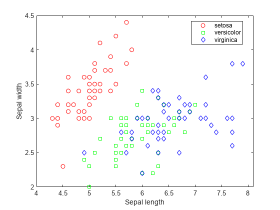
Fisher's iris data consists of measurements on the sepal length, sepal width, petal length, and petal width for 150 iris specimens. There are 50 specimens from each of three species. Load the data and see how the sepal measurements differ between species. You can use the two columns containing sepal measurements.

load fisheriris
f = figure;
gscatter(meas(:,1), meas(:,2), species,'rgb','osd');
xlabel('Sepal length');
ylabel('Sepal width');

N = size(meas,1);

Suppose you measure a sepal and petal from an iris, and you need to determine its species on the basis of those measurements. One approach to solving this problem is known as discriminant analysis.

Linear and Quadratic Discriminant Analysis

The fitcdiscr function can perform classification using different types of discriminant analysis. First classify the data using the default linear discriminant analysis (LDA).

lda = fitcdiscr(meas(:,1:2),species);
ldaClass = resubPredict(lda);

The observations with known class labels are usually called the training data. Now compute the resubstitution error, which is the misclassification error (the proportion of misclassified observations) on the training set.

ldaResubErr = resubLoss(lda)

ldaResubErr = 0.2000

You can also compute the confusion matrix on the training set. A confusion matrix contains information about known class labels and predicted class labels. Generally speaking, the (i,j) element in the confusion matrix is the number of samples whose known class label is class i and whose predicted class is j. The diagonal elements represent correctly classified observations.

figure
ldaResubCM = confusionchart(species,ldaClass);

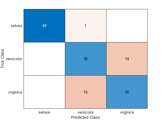
Of the 150 training observations, 20% or 30 observations are misclassified by the linear discriminant function. You can see which ones they are by drawing X through the misclassified points.

figure(f)
bad = ~strcmp(ldaClass,species);
hold on;
plot(meas(bad,1), meas(bad,2), 'kx');
hold off;

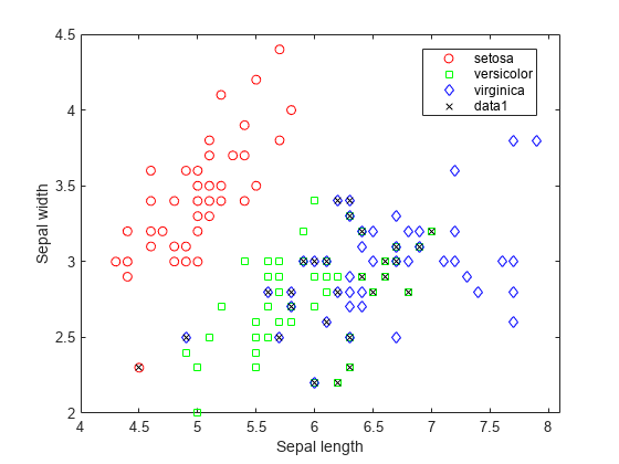
The function has separated the plane into regions divided by lines, and assigned different regions to different species. One way to visualize these regions is to create a grid of (x,y) values and apply the classification function to that grid.

[x,y] = meshgrid(4:.1:8,2:.1:4.5);
x = x(:);
y = y(:);
j = classify([x y],meas(:,1:2),species);
gscatter(x,y,j,'grb','sod')

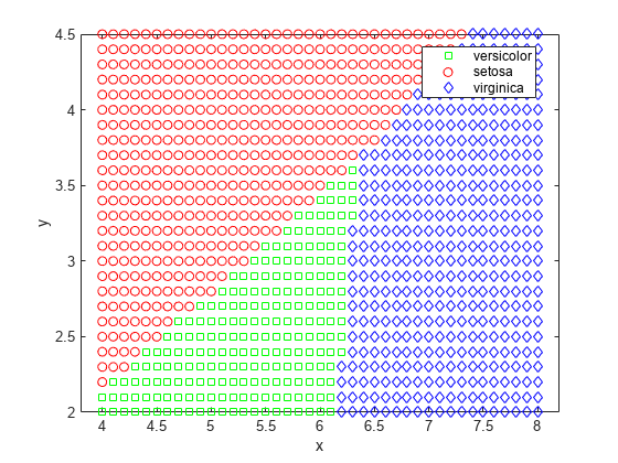
For some data sets, the regions for the various classes are not well separated by lines. When that is the case, linear discriminant analysis is not appropriate. Instead, you can try quadratic discriminant analysis (QDA) for our data.

Compute the resubstitution error for quadratic discriminant analysis.

qda = fitcdiscr(meas(:,1:2),species,'DiscrimType','quadratic');
qdaResubErr = resubLoss(qda)

qdaResubErr = 0.2000

You have computed the resubstitution error. Usually people are more interested in the test error (also referred to as generalization error), which is the expected prediction error on an independent set. In fact, the resubstitution error will likely under-estimate the test error.

In this case you don't have another labeled data set, but you can simulate one by doing cross-validation. A stratified 10-fold cross-validation is a popular choice for estimating the test error on classification algorithms. It randomly divides the training set into 10 disjoint subsets. Each subset has roughly equal size and roughly the same class proportions as in the training set. Remove one subset, train the classification model using the other nine subsets, and use the trained model to classify the removed subset. You could repeat this by removing each of the ten subsets one at a time.

Because cross-validation randomly divides data, its outcome depends on the initial random seed. To reproduce the exact results in this example, execute the following command:

rng(0,'twister');

First use cvpartition to generate 10 disjoint stratified subsets.

cp = cvpartition(species,'KFold',10)

cp = 
K-fold cross validation partition
   NumObservations: 150
       NumTestSets: 10
         TrainSize: 135  135  135  135  135  135  135  135  135  135
          TestSize: 15  15  15  15  15  15  15  15  15  15
          IsCustom: 0

The crossval and kfoldLoss methods can estimate the misclassification error for both LDA and QDA using the given data partition cp.

Estimate the true test error for LDA using 10-fold stratified cross-validation.

cvlda = crossval(lda,'CVPartition',cp);
ldaCVErr = kfoldLoss(cvlda)

ldaCVErr = 0.2000

The LDA cross-validation error has the same value as the LDA resubstitution error on this data.

Estimate the true test error for QDA using 10-fold stratified cross-validation.

cvqda = crossval(qda,'CVPartition',cp);
qdaCVErr = kfoldLoss(cvqda)

qdaCVErr = 0.2200

QDA has a slightly larger cross-validation error than LDA. It shows that a simpler model may get comparable, or better performance than a more complicated model.

Naive Bayes Classifiers

The fitcdiscr function has two other types, 'DiagLinear' and 'DiagQuadratic'. They are similar to 'linear' and 'quadratic', but with diagonal covariance matrix estimates. These diagonal choices are specific examples of a naive Bayes classifier, because they assume the variables are conditionally independent given the class label. Naive Bayes classifiers are among the most popular classifiers. While the assumption of class-conditional independence between variables is not true in general, naive Bayes classifiers have been found to work well in practice on many data sets.

The fitcnb function can be used to create a more general type of naive Bayes classifier.

First model each variable in each class using a Gaussian distribution. You can compute the resubstitution error and the cross-validation error.

nbGau = fitcnb(meas(:,1:2), species);
nbGauResubErr = resubLoss(nbGau)

nbGauResubErr = 0.2200

nbGauCV = crossval(nbGau, 'CVPartition',cp);
nbGauCVErr = kfoldLoss(nbGauCV)

nbGauCVErr = 0.2200

labels = predict(nbGau, [x y]);
gscatter(x,y,labels,'grb','sod')

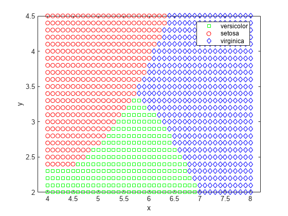
So far you have assumed the variables from each class have a multivariate normal distribution. Often that is a reasonable assumption, but sometimes you may not be willing to make that assumption or you may see clearly that it is not valid. Now try to model each variable in each class using a kernel density estimation, which is a more flexible nonparametric technique. Here we set the kernel to box.

nbKD = fitcnb(meas(:,1:2), species, 'DistributionNames','kernel', 'Kernel','box');
nbKDResubErr = resubLoss(nbKD)

nbKDResubErr = 0.2067

nbKDCV = crossval(nbKD, 'CVPartition',cp);
nbKDCVErr = kfoldLoss(nbKDCV)

nbKDCVErr = 0.2133

labels = predict(nbKD, [x y]);
gscatter(x,y,labels,'rgb','osd')

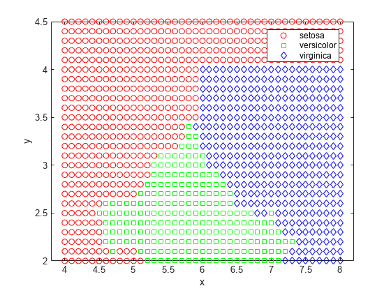
For this data set, the naive Bayes classifier with kernel density estimation gets smaller resubstitution error and cross-validation error than the naive Bayes classifier with a Gaussian distribution.

Decision Tree

Another classification algorithm is based on a decision tree. A decision tree is a set of simple rules, such as "if the sepal length is less than 5.45, classify the specimen as setosa." Decision trees are also nonparametric because they do not require any assumptions about the distribution of the variables in each class.

The fitctree function creates a decision tree. Create a decision tree for the iris data and see how well it classifies the irises into species.

t = fitctree(meas(:,1:2), species,'PredictorNames',{'SL' 'SW' });

It's interesting to see how the decision tree method divides the plane. Use the same technique as above to visualize the regions assigned to each species.

[grpname,node] = predict(t,[x y]);
gscatter(x,y,grpname,'grb','sod')

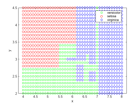
Another way to visualize the decision tree is to draw a diagram of the decision rule and class assignments.

view(t,'Mode','graph');

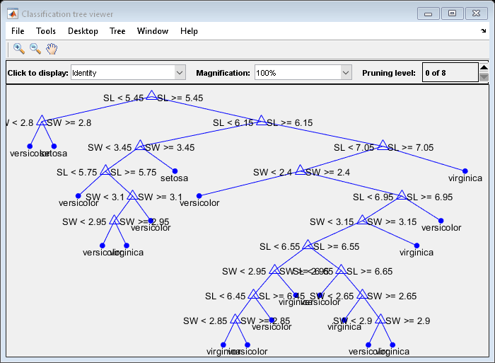
This cluttered-looking tree uses a series of rules of the form "SL < 5.45" to classify each specimen into one of 19 terminal nodes. To determine the species assignment for an observation, start at the top node and apply the rule. If the point satisfies the rule you take the left path, and if not you take the right path. Ultimately you reach a terminal node that assigns the observation to one of the three species.

Compute the resubstitution error and the cross-validation error for decision tree.

dtResubErr = resubLoss(t)

dtResubErr = 0.1333

cvt = crossval(t,'CVPartition',cp);
dtCVErr = kfoldLoss(cvt)

dtCVErr = 0.3000

For the decision tree algorithm, the cross-validation error estimate is significantly larger than the resubstitution error. This shows that the generated tree overfits the training set. In other words, this is a tree that classifies the original training set well, but the structure of the tree is sensitive to this particular training set so that its performance on new data is likely to degrade. It is often possible to find a simpler tree that performs better than a more complex tree on new data.

Try pruning the tree. First compute the resubstitution error for various subsets of the original tree. Then compute the cross-validation error for these sub-trees. A graph shows that the resubstitution error is overly optimistic. It always decreases as the tree size grows, but beyond a certain point, increasing the tree size increases the cross-validation error rate.

resubcost = resubLoss(t,'Subtrees','all');
[cost,secost,ntermnodes,bestlevel] = cvloss(t,'Subtrees','all');
plot(ntermnodes,cost,'b-', ntermnodes,resubcost,'r--')
figure(gcf);
xlabel('Number of terminal nodes');
ylabel('Cost (misclassification error)')
legend('Cross-validation','Resubstitution')

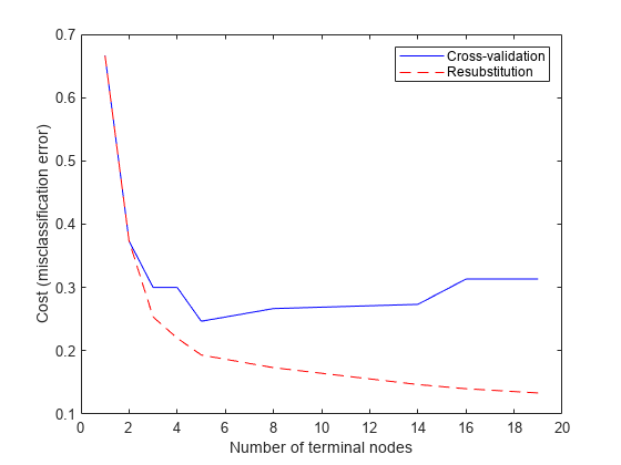
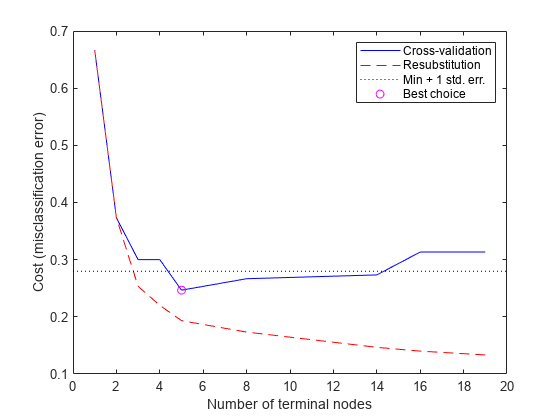
Which tree should you choose? A simple rule would be to choose the tree with the smallest cross-validation error. While this may be satisfactory, you might prefer to use a simpler tree if it is roughly as good as a more complex tree. For this example, take the simplest tree that is within one standard error of the minimum. That's the default rule used by the cvloss method of ClassificationTree.

You can show this on the graph by computing a cutoff value that is equal to the minimum cost plus one standard error. The "best" level computed by the cvloss method is the smallest tree under this cutoff. (Note that bestlevel=0 corresponds to the unpruned tree, so you have to add 1 to use it as an index into the vector outputs from cvloss.)

[mincost,minloc] = min(cost);
cutoff = mincost + secost(minloc);
hold on
plot([0 20], [cutoff cutoff], 'k:')
plot(ntermnodes(bestlevel+1), cost(bestlevel+1), 'mo')
legend('Cross-validation','Resubstitution','Min + 1 std. err.','Best choice')
hold off

Finally, you can look at the pruned tree and compute the estimated misclassification error for it.

pt = prune(t,'Level',bestlevel);
view(pt,'Mode','graph')

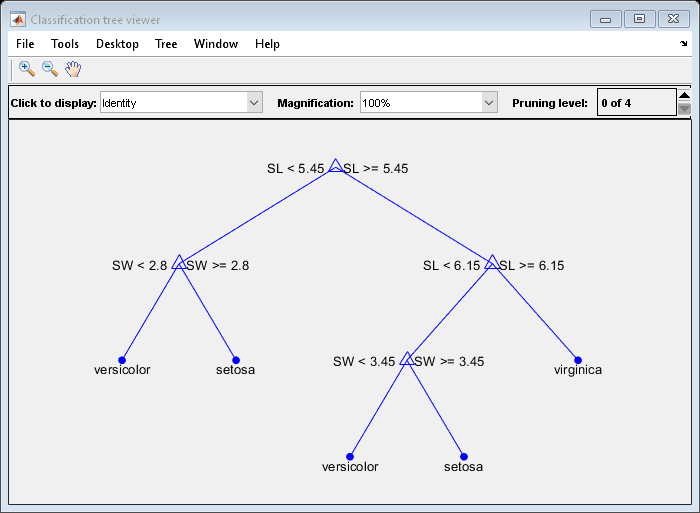
cost(bestlevel+1)

ans = 0.2467

Conclusions

This example shows how to perform classification in MATLAB® using Statistics and Machine Learning Toolbox™ functions.

This example is not meant to be an ideal analysis of the Fisher iris data. In fact, using the petal measurements instead of, or in addition to, the sepal measurements may lead to better classification. Also, this example is not meant to compare the strengths and weaknesses of different classification algorithms. You may find it instructive to perform the analysis on other data sets and compare different algorithms. There are also Toolbox functions that implement other classification algorithms. For instance, you can use TreeBagger to perform bootstrap aggregation for an ensemble of decision trees, as described in the example Bootstrap Aggregation (Bagging) of Classification Trees Using TreeBagger.