dlistft
Description
x = dlistft(y)y. The
dlistft function requires Deep Learning Toolbox™.
x = dlistft(y,Name=Value)DataFormat="CBT" specifies the data
format of y as CBT.
Examples
Deep Learning Inverse Short-Time Fourier Transform
Create a random signal with three channels and 1024 samples representing a batch of 5. Save the signal as a dlarray in "CTB" format. Display the dimension sizes and data format of the array. dlarray permutes the array dimensions to the "CBT" shape expected by a deep learning network.
x = dlarray(randn([3 1024 5]),"CTB");
size(x)
ans = 1×3
3 5 1024
dims(x)
ans =
'CBT'
Compute the short-time Fourier transform (STFT) of the signal using the default dlstft function values. The STFT is a dlarray in "SCBT" format.
ydl = dlstft(x);
dims(ydl)
ans =
'SCBT'
Compute the deep learning inverse short-time Fourier transform using the default dlistft function values. The output is a dlarray in "CBT" format.
X = dlistft(ydl);
dims(X)
ans =
'CBT'
Deep Learning Inverse Short-Time Fourier Transform of Chirp
Generate an N-by-2 matrix. Each column is a quadratic chirp sampled at 8192 Hz for two seconds.
Fs = 8192;
t = 0:1/Fs:2-1/Fs;
Nt = numel(t);
x = repmat(chirp(t,250,1,500,"quadratic")',1,2);
size(x)
ans = 1×2
16384 2
Save the matrix as an unformatted dlarray containing a batch of two single-channel signals. Use the reshape function to insert the third dimension.
x = dlarray(reshape(x,Nt,1,[]));
size(x)
ans = 1×3

       16384           1           2
Obtain the deep learning short-time Fourier transform. Specify a 512-sample Hann window, an FFT length of 600, and an overlap of 384 samples. Specify the format of the input dlarray as "TCB". The output is an unformatted dlarray.
nfft = 600;
winLen = 512;
win = hann(winLen);
noverlap = 384;
fmt = "TCB";
[ydl,fd1,tdl] = dlstft(x,Fs,Window=win,OverlapLength=noverlap, ...
    FFTLength=nfft,DataFormat=fmt);
Compute the deep learning inverse short-time Fourier transform. Specify the data format as "SCBT". To obtain perfect reconstruction, use the same name-value arguments for the ISTFT computation as for the STFT computation. The expected number of channels and samples in the output are 1 and Nt, respectively. The dimension order of the reconstruction is "CBT".
outsize = [1 Nt];
invfmt = "SCBT";
X = dlistft(ydl,Window=win,OverlapLength=noverlap, ...
    FFTLength=nfft,DataFormat=invfmt, ...
    ExpectedOutputSize=outsize);
size(X)
ans = 1×3

           1           2       16384
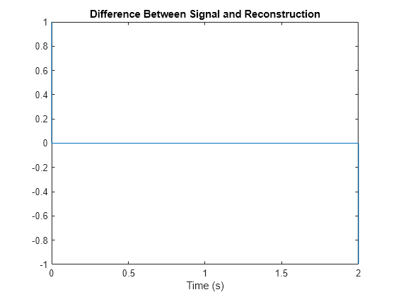
Plot the difference between a single-channel signal and its reconstruction. Except for the end points, the reconstruction is perfect.
idx = 1;
sig = extractdata(x(:,1,idx));
Xp = permute(X,[3 1 2]);
rec = extractdata(Xp(:,1,idx));
plot(t,sig-rec)
title("Difference Between Signal and Reconstruction")
xlabel("Time (s)")

To remove edge effects, zero-pad the original data on both sides along the time dimension. The length of the zero-pad is the window length. Then compute the STFT.
xPadded = paddata(x,Nt+2*winLen,dimension=1,side="both");
ydl = dlstft(xPadded,Fs,Window=win,OverlapLength=noverlap, ...
    FFTLength=nfft,DataFormat=fmt);
Compute the deep learning inverse short-time Fourier transform. The expected number of samples in the output is Nt+2*winLen.
outsize = [1 Nt+2*winLen];
X = dlistft(ydl,Window=win,OverlapLength=noverlap, ...
    FFTLength=nfft,DataFormat=invfmt, ...
    ExpectedOutputSize=outsize);
size(X)
ans = 1×3

           1           2       17408
Trim both sides of the ISTFT output along the time dimension to length Nt.
X = trimdata(X,Nt,dimension=3,side="both");
size(X)
ans = 1×3
1 2 16384
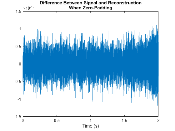
Plot the difference between a single-channel signal and its reconstruction. Because zero-padding the data removes edge effects, the reconstruction is perfect.
idx = 2;
sig = extractdata(x(:,1,idx));
Xp = permute(X,[3 1 2]);
rec = extractdata(Xp(:,1,idx));
plot(t,sig-rec)
title({"Difference Between Signal and Reconstruction", ...
    "When Zero-Padding"})
xlabel("Time (s)")
Concatenating Real and Imaginary Parts of dlistft Input
This example shows how to concatenate the real and imaginary parts of the STFT input to the dlistft function.
Generate a 3-by-160(-by-1) array containing one batch of a three-channel, 160-sample sinusoidal signal. The normalized sinusoid frequencies are π/4 rad/sample, π/2 rad/sample, and 3π/4 rad/sample. Save the signal as a dlarray, specifying the dimensions in order. dlarray permutes the array dimensions to the "CBT" shape expected by a deep learning network. Display the array dimension sizes.
x = dlarray(cos(pi.*(1:3)'/4*(0:159)),'CTB');
[nchan,nbtch,nsamp] = size(x)
nchan = 3
nbtch =
1
nsamp =
160
Compute the deep learning short-time Fourier transform of the signal. Specify a 64-sample rectangular window and an FFT length of 1024. The STFT output is in "SCBT" format. Confirm the output is complex-valued. Display the array dimension sizes of the output.
y = dlstft(x,Window=rectwin(64),FFTLength=1024);
~isreal(y)
ans = logical
   1
size(y)
ans = 1×4

   513     3     1     7
Concatenate the real and imaginary parts of the output along the second dimension.
yr = real(y);
yi = imag(y);
yc = cat(2,yr,yi);
isreal(yc)
ans = logical
   1
size(yc)
ans = 1×4

   513     6     1     7
Obtain the deep learning ISTFT of the concatenated dlarray. Confirm perfect reconstruction of the original data.
xrec = dlistft(yc,Window=rectwin(64),FFTLength=1024);
max(abs(x(:)-xrec(:)))
ans =
  1x1 dlarray

   3.4377e-14
Input Arguments
y — One-sided short-time Fourier transform
dlarray object | numeric array
One-sided short-time Fourier transform, specified as a formatted or unformatted
dlarray (Deep Learning Toolbox) object,
or a numeric array.
If
yis a formatteddlarray, it must be in the"SCBT"or"CBT"format.If
yis in the"CBT"format, the size of the"C"dimension must be divisible byfloor(.FFTLength/2)+1If
yis in the"SCBT"format, the size of the"S"dimension must equalfloor(.FFTLength/2)+1
If
yis in the"CBT"format, thedlistftfunction unflattensyto have shape"SCBT". The"S"dimension corresponds to frequency.If
yis real-valued, the number of channelsCmust be even because thedlistftfunction assumes the true number of channels isC/2. For more information, see Concatenating Real and Imaginary Parts of dlistft Input.If
yis an unformatteddlarrayor a numeric array, it must be compatible with the"SCBT"or"CBT"formats and you must setDataFormat.
Data Types: double | single
Complex Number Support: Yes
Name-Value Arguments
Specify optional pairs of arguments as
Name1=Value1,...,NameN=ValueN, where Name is
the argument name and Value is the corresponding value.
Name-value arguments must appear after other arguments, but the order of the
pairs does not matter.
Example: Window=hamming(100),OverlapLength=50,FFTLength=128,Method="wola"
uses a 100-sample Hamming window, with 50 samples of overlap between adjoining segments and
a 128-point DFT.
DataFormat — Input data format
character vector | string scalar
Input data format, specified as a character vector or string scalar. This argument
is valid only if y is unformatted.
Each character in this argument must be one of these labels:
"S"—Spatial (frequency) dimension"C"— Channel"B"— Batch observations"T"— Time
The dlistft function accepts any permutation of
"CBT" or "SCBT". You can specify at most one
of each of the "S", "C", "B",
and "T" labels.
Each element of the argument labels the matching dimension of
y. When you specify a data format,
dlistft implicitly permutes both the argument and the data
to match this order:
"S""C""B""T"
How the function stores the data remains the same.
Example: "CBT" specifies the format
channel-batch-time.
Window — Windowing function
hann(128,"periodic") (default) | vector | dlarray object
Windowing function, specified as a vector or a dlarray object.
The length of Window must be greater than or equal to 2. For a
list of available windows, see Windows.
For perfect time-domain reconstruction, the window for the ISTFT computation must
match the window for the STFT computation. Use the function iscola to
check a window/overlap combination for constant overlap-add (COLA) compliance. COLA
compliance is a requirement for perfect reconstruction for non-modified spectra. For
more information, see Constant Overlap-Add (COLA) Constraint. If the window is a dlarray object, extract data from the
dlarray before using the iscola
function.
Example: hann(N+1) and
(1-cos(2*pi*(0:N)'/N))/2 both specify a Hann window of length
N + 1, where N is a positive
integer.
Data Types: double | single
OverlapLength — Number of overlapped samples
75% of window length (default) | nonnegative integer
Number of overlapped samples between adjoining segments, specified as a
nonnegative integer smaller than the length of Window. If you
omit OverlapLength or specify it as empty, the function sets it
to the largest integer less than 75% of the window length, which turns out to be 96
samples for the default Hann window.
Data Types: double | single
FFTLength — Number of DFT points
window length (default) | positive integer
Number of DFT points, specified as a positive integer.
FFTLength must be greater than or equal to the window length.
You must specify the same number of DFT points for the STFT and
ISTFT.
Data Types: double | single
Method — Method of overlap-add
"wola" (default) | "ola"
Method of overlap-add, specified as one of these:
"wola"— Weighted overlap-add"ola"— Overlap-add
For more information, see Constant Overlap-Add (COLA) Constraint.
ExpectedOutputSize — Expected number of channels and samples
two-element vector
Expected number of channels and samples in the reconstructed signal, specified as a two-element vector of positive integers. The first element is the expected number of channels and the second element is the expected number of time samples.
By default, dlistft does not check the size of the output. To
perform size validation, set ExpectedOutputSize. When you set
ExpectedOutputSize, dlistft validates
the expected size before computing the ISTFT. The function errors if the validation
does not pass. For more information, see Algorithms.
Data Types: single | double
Output Arguments
x — Reconstructed signal
dlarray object
Reconstructed signal, returned as a formatted or unformatted
dlarray object.
If
yis a formatteddlarray, thenxis a"CBT"formatteddlarray.If
yis an unformatteddlarray, thenxis an unformatteddlarray. The dimension order inxis"CBT".
The dlistft function computes the inverse short-time
Fourier transform along the "S" dimension of y.
For perfect reconstruction for non-modified spectra, the window must be COLA compliant.
For more information, see Constant Overlap-Add (COLA) Constraint.
More About
Inverse Short-Time Fourier Transform
The inverse short-time Fourier transform is computed by taking the IFFT of each DFT vector of the STFT and overlap-adding the inverted signals.
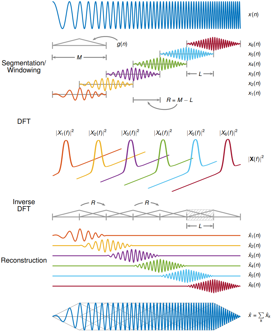
Recall that the STFT of a signal is computed by sliding an analysis window g(n) of length M over the signal and calculating the discrete Fourier transform (DFT) of each segment of windowed data. The window hops over the original signal at intervals of R samples, equivalent to L = M – R samples of overlap between adjoining segments. The ISTFT is calculated as follows.
where is the DFT of the windowed data centered about time and . The inverse STFT is a perfect reconstruction of the original signal as long as where is a nonzero constant and equals 0 or 1. For more information, see Constant Overlap-Add (COLA) Constraint. This figure depicts the steps in reconstructing the original signal.

Constant Overlap-Add (COLA) Constraint
To ensure successful reconstruction of nonmodified spectra, the analysis window must satisfy the COLA constraint. In general, if the analysis window satisfies the condition where is a nonzero constant and equals 0 or 1, the window is considered to be COLA-compliant. Additionally, COLA compliance can be described as either weak or strong.
Weak COLA compliance implies that the Fourier transform of the analysis window has zeros at frame-rate harmonics such that
Alias cancellation is disturbed by spectral modifications. Weak COLA relies on alias cancellation in the frequency domain. Therefore, perfect reconstruction is possible using weakly COLA-compliant windows as long as the signal has not undergone any spectral modifications.
For strong COLA compliance, the Fourier transform of the window must be bandlimited consistently with downsampling by the frame rate such that
This equation shows that no aliasing is allowed by the strong COLA constraint. Additionally, for strong COLA compliance, the value of the constant must equal 1. In general, if the short-time spectrum is modified in any way, a stronger COLA compliant window is preferred.
You can use the iscola function to check for weak COLA compliance. The number of summations used to check COLA compliance is dictated by the window length and hop size. In general, it is common to use in for weighted overlap-add (WOLA), and for overlap-add (OLA). By default, istft uses the WOLA method, by applying a synthesis window before performing the overlap-add method.
In general, the synthesis window is the same as the analysis window. You can construct useful WOLA windows by taking the square root of a strong OLA window. You can use this method for all nonnegative OLA windows. For example, the root-Hann window is a good example of a WOLA window.
Perfect Reconstruction
In general, computing the STFT of an input signal and inverting it does not result in perfect reconstruction. If you want the output of ISTFT to match the original input signal as closely as possible, the signal and the window must satisfy the following conditions:
Input size — If you invert the output of
stftusingistftand want the result to be the same length as the input signalx, the value ofmust be an integer. In the equation, Nx is the length of the signal, M is the length of the window, and L is the overlap length.
COLA compliance — Use COLA-compliant windows, assuming that you have not modified the short-time Fourier transform of the signal.
Padding — If the length of the input signal is such that the value of k is not an integer, zero-pad the signal before computing the short-time Fourier transform. Remove the extra zeros after inverting the signal.
You can use the stftmag2sig
function to obtain an estimate of a signal reconstructed from the magnitude of its
STFT.
Algorithms
If you set ExpectedOutputSize, the dlistft
function computes the number of channels and samples in the reconstruction before performing
the ISTFT. If the values do not match ExpectedOutputSize, the function
errors. The size of the reconstruction depends on the dimensions, and data format of the input
STFT, the length of the windowing function, the number of overlapped samples and the number of
DFT points.
dlistft determines the number of channels and samples as follows.
Define the hop size as hopSize =
length(.Window)-OverlapLength
If
yis a"SCBT"formatteddlarray, or an unformatteddlarraycompatible with"SCBT"format:If
yis complex-valued, the number of channels issize(. Otherwise, the number of channels isy,2)size(.y,2)/2The number of samples is
length(, whereWindow)+(nseg-1)*hopSizenseg = size(.y,4)
If
yis a"CBT"formatteddlarray, or an unformatteddlarraycompatible with"CBT"format:If
yis complex-valued, the number of channels issize(, wherey,1)/nfreqnfreq = floor(. Otherwise, the number of channels isFFTLength/2)+1size(.y,1)/(2*nfreq)The number of samples is
length(, whereWindow)+(nseg-1)*hopSizenseg = size(.y,3)
Extended Capabilities
GPU Arrays
Accelerate code by running on a graphics processing unit (GPU) using Parallel Computing Toolbox™.
This function fully supports GPU arrays. For more information, see Run MATLAB Functions on a GPU (Parallel Computing Toolbox).
Version History
Introduced in R2024a
See Also
Objects
stftLayer|istftLayer|dlarray(Deep Learning Toolbox)
Functions
dlstft|stft|istft|iscola|stftmag2sig
MATLAB Command
You clicked a link that corresponds to this MATLAB command:
Run the command by entering it in the MATLAB Command Window. Web browsers do not support MATLAB commands.

Select a Web Site
Choose a web site to get translated content where available and see local events and offers. Based on your location, we recommend that you select: .
You can also select a web site from the following list
How to Get Best Site Performance
Select the China site (in Chinese or English) for best site performance. Other bat365 country sites are not optimized for visits from your location.
Americas
- América Latina (Español)
- Canada (English)
- United States (English)
Europe
- Belgium (English)
- Denmark (English)
- Deutschland (Deutsch)
- España (Español)
- Finland (English)
- France (Français)
- Ireland (English)
- Italia (Italiano)
- Luxembourg (English)
- Netherlands (English)
- Norway (English)
- Österreich (Deutsch)
- Portugal (English)
- Sweden (English)
- Switzerland
- United Kingdom (English)
Asia Pacific
- Australia (English)
- India (English)
- New Zealand (English)
- 中国
- 日本Japanese (日本語)
- 한국Korean (한국어)