Train SAC Agent for Ball Balance Control
This example shows how to train a soft actor-critic (SAC) reinforcement learning agent to control a robot arm for a ball-balancing task.
Introduction
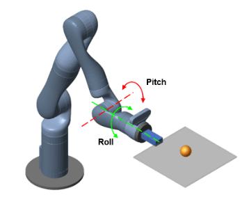
The robot arm in this example is a Kinova Gen3 robot, which is a seven degree-of-freedom (DOF) manipulator. The arm is tasked to balance a ping pong ball at the center of a flat surface (plate) attached to the robot gripper. Only the final two joints are actuated and contribute to motion in the pitch and roll axes as shown in the following figure. The remaining joints are fixed and do not contribute to motion.
Open the Simulink® model to view the system. The model contains a Kinova Ball Balance subsystem connected to an RL Agent block. The agent applies an action to the robot subsystem and receives the resulting observation, reward, and is-done signals.
open_system("rlKinovaBallBalance")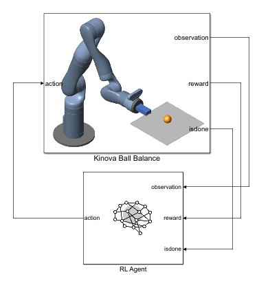
View to the Kinova Ball Balance subsystem.
open_system("rlKinovaBallBalance/Kinova Ball Balance")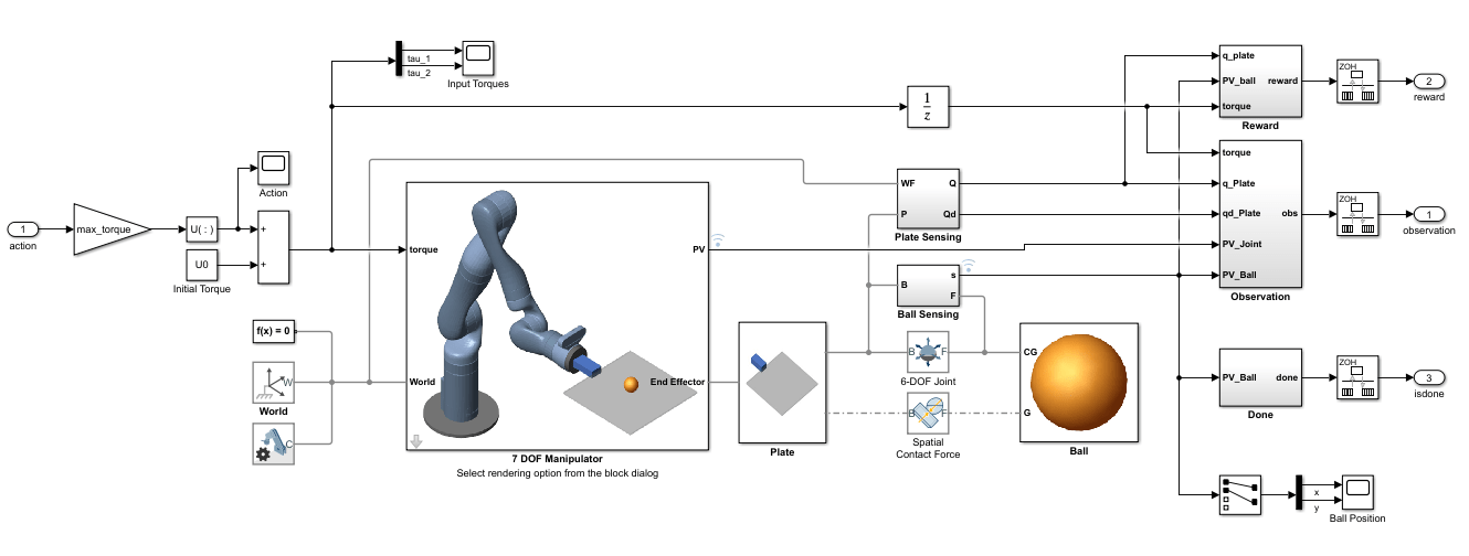
In this model:
The physical components of the system (manipulator, ball, and plate) are modeled using Simscape™ Multibody™ components.
The plate is constrained to the end effector of the manipulator.
The ball has six degrees of freedom and can move freely in space.
Contact forces between the ball and plate are modeled using the Spatial Contact Force block.
Control inputs to the manipulator are the torque signals for the actuated joints.
If you have the Robotics System Toolbox Robot Library Data support package, you can view a 3-D animation of the manipulator in the Mechanics Explorer. To do so, open the 7 DOF Manipulator subsystem and set its Visualization parameter to 3D Mesh. If you do have the support package installed, set the Visualization parameter to None. To download and install the support package, use the Add-On Explorer. For more information see Get and Manage Add-Ons.
Create the parameters for the example by running the kinova_params script included with this example. When you have the Robotics System Toolbox Robot Library Data support package installed, this script also adds the necessary mesh files to the MATLAB® path.
kinova_params
Define Environment
To train a reinforcement learning agent, you must define the environment with which it will interact. For the ball balancing environment:
The observations are represented by a 22 element vector that contains information about the positions (sine and cosine of joint angles) and velocities (joint angle derivatives) of the two actuated joints, positions (x and y distances from plate center) and velocities (x and y derivatives) of the ball, orientation (quaternions) and velocities (quaternion derivatives) of the plate, joint torques from the last time step, ball radius, and mass.
The actions are normalized joint torque values.
The sample time is , and the simulation time is .
The simulation terminates when the ball falls off the plate.
The reward at time step is given by:
Here, is a reward for the ball moving closer to the center of the plate, is a penalty for plate orientation, and is a penalty for control effort. , , and are the respective roll, pitch, and yaw angles of the plate in radians. and are the joint torques.
Create the observation and action specifications for the environment using continuous observation and action spaces.
numObs = 22;  % Number of dimension of the observation space
numAct = 2;   % Number of dimension of the action space

obsInfo = rlNumericSpec([numObs 1]);

actInfo = rlNumericSpec([numAct 1]);
actInfo.LowerLimit = -1;
actInfo.UpperLimit = 1;
Create the Simulink environment interface using the observation and action specifications. For more information on creating Simulink environments, see rlSimulinkEnv.
mdl = "rlKinovaBallBalance";
blk = mdl + "/RL Agent";
env = rlSimulinkEnv(mdl,blk,obsInfo,actInfo);
Specify a reset function for the environment using the ResetFcn parameter.
env.ResetFcn = @kinovaResetFcn;
This reset function (provided at the end of this example) randomly initializes the initial x and y positions of the ball with respect to the center of the plate. For more robust training, you can also randomize other parameters inside the reset function, such as the mass and radius of the ball.
Specify the sample time Ts and simulation time Tf.
Ts = 0.01;
Tf = 10;
Create Agent
The agent in this example is a soft actor-critic (SAC) agent. SAC agents use one or two parametrized Q-value function approximators to estimate the value of the policy. A Q-value function critic takes the current observation and an action as inputs and returns a single scalar as output (the estimated discounted cumulative long-term reward for which receives the action from the state corresponding to the current observation, and following the policy thereafter). For more information on SAC agents, see Soft Actor-Critic (SAC) Agents.
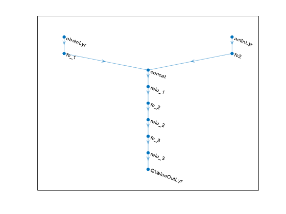
The SAC agent in this example uses two critics. To model the parametrized Q-value functions within the critics, use a neural network with two input layers (one for the observation channel, as specified by obsInfo, and the other for the action channel, as specified by actInfo) and one output layer (which returns the scalar value).
Define each network path as an array of layer objects. Assign names to the input and output layers of each path. These names allow you to connect the paths and then later explicitly associate the network input and output layers with the appropriate environment channel.
For more information on creating deep neural networks for reinforcement learning agents, see Create Policies and Value Functions.
% Set the random seed for reproducibility.
rng(0)

% Define the network layers.
criticNet = [
    featureInputLayer(numObs,Name="obsInLyr")
    fullyConnectedLayer(128)
    concatenationLayer(1,2,Name="concat")
    reluLayer
    fullyConnectedLayer(64)
    reluLayer
    fullyConnectedLayer(32)
    reluLayer
    fullyConnectedLayer(1,Name="QValueOutLyr")
    ];

actionPath = [
    featureInputLayer(numAct,Name="actInLyr")
    fullyConnectedLayer(128,Name="fc2")
    ];

% Connect the layers.
criticNet = layerGraph(criticNet);
criticNet = addLayers(criticNet, actionPath);
criticNet = connectLayers(criticNet,"fc2","concat/in2");
View the critic neural network.
plot(criticNet)
When using two critics, a SAC agent requires them to have different initial parameters. Create and initialize two dlnetwork objects.
criticDLnet = dlnetwork(criticNet,'Initialize',false);
criticDLnet1 = initialize(criticDLnet);
criticDLnet2 = initialize(criticDLnet);
Create the critic functions using rlQValueFunction.
critic1 = rlQValueFunction(criticDLnet1,obsInfo,actInfo, ...
    ObservationInputNames="obsInLyr");
critic2 = rlQValueFunction(criticDLnet2,obsInfo,actInfo, ...
    ObservationInputNames="obsInLyr");
Soft Actor-critic agents use a parametrized stochastic policy over a continuous action space, which is implemented by a continuous Gaussian actor.
This actor takes an observation as input and returns as output a random action sampled from a Gaussian probability distribution.
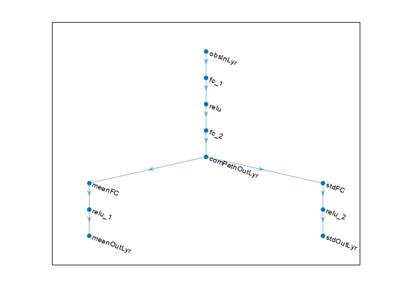
To approximate the mean values and standard deviations of the Gaussian distribution, you must use a neural network with two output layers, each having as many elements as the dimension of the action space. One output layer must return a vector containing the mean values for each action dimension. The other must return a vector containing the standard deviation for each action dimension.
Since standard deviations must be nonnegative, use a softplus or ReLU layer to enforce nonnegativity. The SAC agent automatically reads the action range from the UpperLimit and LowerLimit properties of actInfo (which is used to create the actor), and then internally scales the distribution and bounds the action. Therefore, do not add a tanhLayer as the last nonlinear layer in the mean output path.
Define each network path as an array of layer objects, and assign names to the input and output layers of each path.
% Create the actor network layers.
commonPath = [
    featureInputLayer(numObs,Name="obsInLyr")
    fullyConnectedLayer(128)
    reluLayer
    fullyConnectedLayer(64)
    reluLayer(Name="comPathOutLyr")
    ];

meanPath = [
    fullyConnectedLayer(32,Name="meanFC")
    reluLayer
    fullyConnectedLayer(numAct,Name="meanOutLyr")
    ];

stdPath = [
    fullyConnectedLayer(numAct,Name="stdFC")
    reluLayer
    softplusLayer(Name="stdOutLyr")
    ];

% Connect the layers.
actorNetwork = layerGraph(commonPath);
actorNetwork = addLayers(actorNetwork,meanPath);
actorNetwork = addLayers(actorNetwork,stdPath);
actorNetwork = connectLayers(actorNetwork,"comPathOutLyr","meanFC/in");
actorNetwork = connectLayers(actorNetwork,"comPathOutLyr","stdFC/in");
View the actor neural network.
plot(actorNetwork)
Create the actor function using rlContinuousGaussianActor.
actordlnet = dlnetwork(actorNetwork);
actor = rlContinuousGaussianActor(actordlnet, obsInfo, actInfo, ...
    ObservationInputNames="obsInLyr", ...
    ActionMeanOutputNames="meanOutLyr", ...
    ActionStandardDeviationOutputNames="stdOutLyr");
The SAC agent in this example trains from an experience buffer of maximum capacity 1e6 by randomly selecting mini-batches of size 128. The fact that the discount factor is 0.99, that is very close to 1, means that the agent keeps more into account long term rewards (a discount factor closer to 0 would instead place a heavier discount on future rewards, therefore encouraging short term ones). For a full list of SAC hyperparameters and their descriptions, see rlSACAgentOptions.
Specify the agent hyperparameters for training.
agentOpts = rlSACAgentOptions( ...
    SampleTime=Ts, ...
    TargetSmoothFactor=1e-3, ...
    ExperienceBufferLength=1e6, ...
    MiniBatchSize=128, ...
    NumWarmStartSteps=1000, ...
    DiscountFactor=0.99);
For this example the actor and critic neural networks are updated using the Adam algorithm with a learn rate of 1e-4 and gradient threshold of 1. Specify the optimizer parameters.
agentOpts.ActorOptimizerOptions.Algorithm = "adam";
agentOpts.ActorOptimizerOptions.LearnRate = 1e-4;
agentOpts.ActorOptimizerOptions.GradientThreshold = 1;

for ct = 1:2
    agentOpts.CriticOptimizerOptions(ct).Algorithm = "adam";
    agentOpts.CriticOptimizerOptions(ct).LearnRate = 1e-4;
    agentOpts.CriticOptimizerOptions(ct).GradientThreshold = 1;
end
Create the SAC agent.
agent = rlSACAgent(actor,[critic1,critic2],agentOpts);
Train Agent
To train the agent, first specify the training options using rlTrainingOptions. For this example, use the following options:
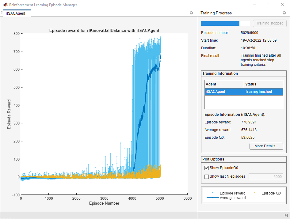
Run each training for at most 5000 episodes, with each episode lasting at most
floor(Tf/Ts)time steps.Stop training when the agent receives an average cumulative reward greater than 675 over 100 consecutive episodes.
To speed up training set the
UseParalleloption totrue, which requires Parallel Computing Toolbox™ software. If you do not have the software installed set the option tofalse.
trainOpts = rlTrainingOptions(...
    MaxEpisodes=6000, ...
    MaxStepsPerEpisode=floor(Tf/Ts), ...
    ScoreAveragingWindowLength=100, ...
    Plots="training-progress", ...
    StopTrainingCriteria="AverageReward", ...
    StopTrainingValue=675, ...
    UseParallel=false);
Specify a visualization flag doViz that shows animation of the ball in a MATLAB figure. For parallel training, disable all visualization.
if trainOpts.UseParallel
    % Disable visualization in Simscape Mechanics Explorer
    set_param(mdl, SimMechanicsOpenEditorOnUpdate="off");
    set_param(mdl+"/Kinova Ball Balance/7 DOF Manipulator", ...
        "VChoice", "None");
    % Disable animation in MATLAB figure
    doViz = false;
    save_system(mdl);
else
    % Enable visualization in Simscape Mechanics Explorer
    set_param(mdl, SimMechanicsOpenEditorOnUpdate="on");
    % Enable animation in MATLAB figure
    doViz = true;
end
You can log training data to disk using the rlDataLogger function. For this example, log the episode experience and actor and critic function losses. The functions logAgentLearnData and logEpisodeData are defined at the end of this Live Script. For more information see Log Training Data to Disk.
logger = rlDataLogger();
logger.AgentLearnFinishedFcn = @logAgentLearnData;
logger.EpisodeFinishedFcn    = @(data) logEpisodeData(data, doViz);
Train the agent using the train function. Training this agent is a computationally intensive process that takes several minutes to complete. To save time while running this example, load a pretrained agent by setting doTraining to false. To train the agent yourself, set doTraining to true.
doTraining = false;
if doTraining
    trainResult = train(agent,env,trainOpts,Logger=logger);
else
    load("kinovaBallBalanceAgent.mat")
end
A snapshot of training progress is shown in the following figure. You can expect different results due to randomness in the training process.
Simulate Trained Agent
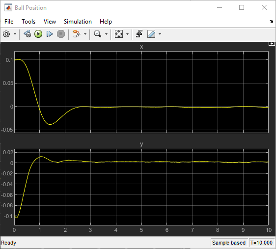
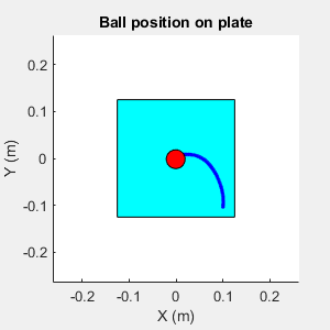
Specify an initial position for the ball with respect to the plate center. To randomize the initial ball position during simulation, set the userSpecifiedConditions flag to false.
userSpecifiedConditions = true;
if userSpecifiedConditions
    ball.x0 = 0.10;
    ball.y0 = -0.10;
    env.ResetFcn = [];
else
    env.ResetFcn = @kinovaResetFcn;
end
Create a simulation options object for configuring the simulation. The agent will be simulated for a maximum of floor(Tf/Ts) steps per simulation episode.
simOpts = rlSimulationOptions(MaxSteps=floor(Tf/Ts));
Enable visualization during simulation.
set_param(mdl, SimMechanicsOpenEditorOnUpdate="on");
doViz = true;
Simulate the agent.
experiences = sim(agent,env,simOpts);
View the trajectory of the ball using the Ball Position scope block.
View the animation of the ball on the plate in a MATLAB figure.
fig = animatedPath(experiences);
Environment Reset Function
function in = kinovaResetFcn(in)
    % KinovaResetFcn is used to randomize the initial joint angles R6_q0,
    % R7_q0 and the initial wrist and hand torque values.

    % Ball parameters
    ball.radius = 0.02;     % m
    ball.mass   = 0.0027;   % kg
    ball.shell  = 0.0002;   % m

    % Calculate ball moment of inertia.
    ball.moi = calcMOI(ball.radius,ball.shell,ball.mass);

    % Initial conditions. +z is vertically upward.
    % Randomize the x and y distances within the plate.
    ball.x0  = -0.125 + 0.25*rand;  % m, initial x distance from plate center
    ball.y0  = -0.125 + 0.25*rand;  % m, initial y distance from plate center
    ball.z0  = ball.radius;         % m, initial z height from plate surface

    ball.dx0 = 0;   % m/s, ball initial x velocity
    ball.dy0 = 0;   % m/s, ball initial y velocity
    ball.dz0 = 0;   % m/s, ball initial z velocity

    % Contact friction parameters
    ball.staticfriction     = 0.5;
    ball.dynamicfriction    = 0.3;
    ball.criticalvelocity   = 1e-3;

    % Convert coefficient of restitution to spring-damper parameters.
    coeff_restitution = 0.89;
    [k, c, w] = cor2SpringDamperParams(coeff_restitution,ball.mass);
    ball.stiffness = k;
    ball.damping = c;
    ball.transitionwidth = w;

    in = setVariable(in,"ball",ball);

    % Randomize joint angles within a range of +/- 5 deg from the
    % starting positions of the joints.
    R6_q0 = deg2rad(-65) + deg2rad(-5+10*rand);
    R7_q0 = deg2rad(-90) + deg2rad(-5+10*rand);
    in = setVariable(in,"R6_q0",R6_q0);
    in = setVariable(in,"R7_q0",R7_q0);

    % Compute approximate initial joint torques that hold the ball,
    % plate and arm at their initial congifuration
    g = 9.80665;
    wrist_torque_0 = ...
        (-1.882 + ball.x0 * ball.mass * g) * cos(deg2rad(-65) - R6_q0);
    hand_torque_0 = ...
        (0.0002349 - ball.y0 * ball.mass * g) * cos(deg2rad(-90) - R7_q0);
    U0 = [wrist_torque_0 hand_torque_0];
    in = setVariable(in,"U0",U0);
end
Data Logging Functions
function dataToLog = logAgentLearnData(data)
% This function is executed after completion
% of the agent's learning subroutine

dataToLog.ActorLoss = data.ActorLoss;
dataToLog.CriticLoss = data.CriticLoss;

end

function dataToLog = logEpisodeData(data, doViz)
% This function is executed after the completion of an episode

dataToLog.Experience = data.Experience;

% Show an animation after episode completion
if doViz
    animatedPath(data.Experience);
end

end
See Also
Functions
train|sim|rlSimulinkEnv
Objects
Blocks
Related Examples
- Train Biped Robot to Walk Using Reinforcement Learning Agents
- Control Robot Manipulator Using Passivity-Based Nonlinear MPC (Model Predictive Control Toolbox)
