Introduction

Target classification is an important function in modern radar systems. This example uses machine and deep learning to classify radar echoes from a cylinder and a cone. Although this example uses the synthesized I/Q samples, the workflow is applicable to real radar returns.

RCS Synthesis

The next section shows how to create synthesized data to train the learning algorithms.

The following code simulates the RCS pattern of a cylinder with a radius of 1 meter and a height of 10 meters. The operating frequency of the radar is 850 MHz.

c = 3e8;
fc = 850e6;
[cylrcs,az,el] = rcscylinder(1,1,10,c,fc);
helperTargetRCSPatternPlot(az,el,cylrcs);

The pattern can then be applied to a backscatter radar target to simulate returns from different aspects angles.

cyltgt = phased.BackscatterRadarTarget('PropagationSpeed',c,...
    'OperatingFrequency',fc,'AzimuthAngles',az,'ElevationAngles',el,'RCSPattern',cylrcs);

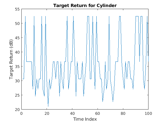
The following plot shows how to simulate 100 returns of the cylinder over time. It is assumed that the cylinder under goes a motion that causes small vibrations around bore sight, as a result, the aspect angle changes from one sample to the next.

rng default;
N = 100;
az = 2*randn(1,N);                  
el = 2*randn(1,N);
cylrtn = cyltgt(ones(1,N),[az;el]);  


plot(mag2db(abs(cylrtn)));
xlabel('Time Index')
ylabel('Target Return (dB)');
title('Target Return for Cylinder');

The return of the cone can be generated similarly. To create the training set, the above process is repeated for 5 arbitrarily selected cylinder radii. In addition, for each radius, 10 motion profiles are simulated by varying the incident angle following 10 randomly generated sinusoid curve around boresight. There are 701 samples in each motion profile, so there are 701-by-50 samples. The process is repeated for the cylinder target, which results in a 701-by-100 matrix of training data with 50 cylinder and 50 cone profiles. In the test set, we use 25 cylinder and 25 cone profiles to create a 701-by-50 training set. Because of the long computation time, the training data is precomputed and loaded below.

load('RCSClassificationReturnsTraining');
load('RCSClassificationReturnsTest');

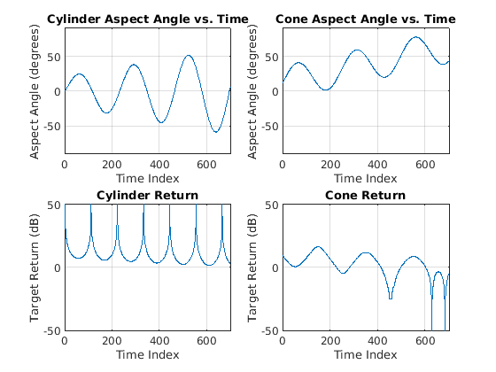
As an example, the next plot shows the return for one of the motion profiles from each shape. The plots show how the values change over time for both the incident azimuth angles and the target returns.

subplot(2,2,1)
plot(cylinderAspectAngle(1,:))
ylim([-90 90])
grid on
title('Cylinder Aspect Angle vs. Time'); xlabel('Time Index'); ylabel('Aspect Angle (degrees)');
subplot(2,2,3)
plot(RCSReturns.Cylinder_1); ylim([-50 50]);
grid on
title('Cylinder Return'); xlabel('Time Index'); ylabel('Target Return (dB)');
subplot(2,2,2)
plot(coneAspectAngle(1,:)); ylim([-90 90]); grid on;
title('Cone Aspect Angle vs. Time'); xlabel('Time Index'); ylabel('Aspect Angle (degrees)');
subplot(2,2,4);
plot(RCSReturns.Cone_1); ylim([-50 50]); grid on;
title('Cone Return'); xlabel('Time Index'); ylabel('Target Return (dB)');

Wavelet Scattering

In the wavelet scattering feature extractor, data is propagated through a series of wavelet transforms, nonlinearities, and averaging to produce low-variance representations of time series. Wavelet time scattering yields signal representations insensitive to shifts in the input signal without sacrificing class discriminability.

The key parameters to specify in a wavelet time scattering network are the scale of the time invariant, the number of wavelet transforms, and the number of wavelets per octave in each of the wavelet filter banks. In many applications, the cascade of two filter banks is sufficient to achieve good performance. In this example, we construct a wavelet time scattering network with the two filter banks: 4 wavelets per octave in the first filter bank and 2 wavelets per octave in the second filter bank. The invariance scale is set to 701 samples, the length of the data.

sn = waveletScattering('SignalLength',701,'InvarianceScale',701,'QualityFactors',[4 2]);

Next, we obtain the scattering transforms of both the training and test sets.

sTrain = sn.featureMatrix(RCSReturns{:,:},'transform','log');
sTest = sn.featureMatrix(RCSReturnsTest{:,:},'transform','log');

For this example, use the mean of the scattering coefficients taken along each path.

TrainFeatures = squeeze(mean(sTrain,2))';
TestFeatures = squeeze(mean(sTest,2))';

Create the labels for training and learning

TrainLabels = repelem(categorical({'Cylinder','Cone'}),[50 50])';
TestLabels = repelem(categorical({'Cylinder','Cone'}),[25 25])';

Model Training

Fit a support vector machine model with a quadratic kernel to the scattering features and obtain the cross-validation accuracy.

template = templateSVM('KernelFunction', 'polynomial', ...
    'PolynomialOrder', 2, ...
    'KernelScale', 'auto', ...
    'BoxConstraint', 1, ...
    'Standardize', true);
classificationSVM = fitcecoc(...
    TrainFeatures, ...
    TrainLabels, ...
    'Learners', template, ...
    'Coding', 'onevsone', ...
    'ClassNames', categorical({'Cylinder','Cone'}));
partitionedModel = crossval(classificationSVM, 'KFold', 5);
[validationPredictions, validationScores] = kfoldPredict(partitionedModel);
validationAccuracy = (1 - kfoldLoss(partitionedModel, 'LossFun', 'ClassifError'))*100

validationAccuracy = 100

Target Classification

Using the trained SVM, classify the scattering features obtained from the test set.

predLabels = predict(classificationSVM,TestFeatures);
accuracy = sum(predLabels == TestLabels )/numel(TestLabels)*100

accuracy = 100

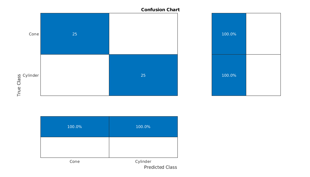
Plot the confusion matrix.

figure('Units','normalized','Position',[0.2 0.2 0.5 0.5]);
ccDCNN = confusionchart(TestLabels,predLabels);
ccDCNN.Title = 'Confusion Chart';
ccDCNN.ColumnSummary = 'column-normalized';
ccDCNN.RowSummary = 'row-normalized';

For more complex data sets, a deep learning workflow may improve performance.

Transfer Learning with a CNN

SqueezeNet is a deep convolutional neural network (CNN) trained for images in 1,000 classes as used in the ImageNet Large Scale Visual Recognition Challenge (ILSVRC). In this example, we reuse the pre-trained SqueezeNet to classify radar returns belonging to one of two classes.

Load SqueezeNet.

snet = squeezenet;

SqueezeNet consists of 68 layers. Like all DCNNs, SqueezeNet cascades convolutional operators followed by nonlinearities and pooling, or averaging. SqueezeNet expects an image input of size 227-by-227-by-3, which you can see with the following code.

snet.Layers(1)

ans = 
  ImageInputLayer with properties:

                      Name: 'data'
                 InputSize: [227 227 3]

   Hyperparameters
          DataAugmentation: 'none'
             Normalization: 'zerocenter'
    NormalizationDimension: 'auto'
                      Mean: [1×1×3 single]

Additionally, SqueezeNet is configured to recognized 1,000 different classes, which you can see with the following code.

snet.Layers(68)

ans = 
  ClassificationOutputLayer with properties:

            Name: 'ClassificationLayer_predictions'
         Classes: [1000×1 categorical]
    ClassWeights: 'none'
      OutputSize: 1000

   Hyperparameters
    LossFunction: 'crossentropyex'

In a subsequent section, we will modify select layers of SqueezeNet in order to apply it to our classification problem.

Continuous Wavelet Transform

SqueezeNet is designed to discriminate differences in images and classify the results. Therefore, in order to use SqueezeNet to classify radar returns, we must transform the 1-D radar return time series into an image. A common way to do this is to use a time-frequency representation (TFR). There are a number of choices for a time-frequency representation of a signal and which one is most appropriate depends on the signal characteristics. To determine which TFR may be appropriate for this problem, randomly choose and plot a few radar returns from each class.

rng default;
idxCylinder = randperm(50,2);
idxCone = randperm(50,2)+50;

It is evident that the radar returns previously shown are characterized by slowing varying changes punctuated by large transient decreases as described earlier. A wavelet transform is ideally suited to sparsely representing such signals. Wavelets shrink to localize transient phenomena with high temporal resolution and stretch to capture slowly varying signal structure. Obtain and plot the continuous wavelet transform of one of the cylinder returns.

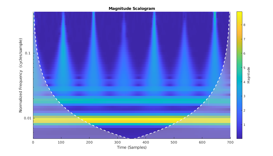
cwt(RCSReturns{:,idxCylinder(1)},'VoicesPerOctave',8)

The CWT simultaneously captures both the slowly varying (low frequency) fluctuations and the transient phenomena. Contrast the CWT of the cylinder return with one from a cone target.

cwt(RCSReturns{:,idxCone(2)},'VoicesPerOctave',8);

Because of the apparent importance of the transients in determining whether the target return originates from a cylinder or cone target, we select the CWT as the ideal TFR to use. After obtaining the CWT for each target return, we make images from the CWT of each radar return. These images are resized to be compatible with SqueezeNet's input layer and we leverage SqueezeNet to classify the resulting images.

Image Preparation

The helper function, helpergenWaveletTFImg, obtains the CWT for each radar return, reshapes the CWT to be compatible with SqueezeNet, and writes the CWT as a jpeg file. To run helpergenWaveletTFImg, choose a parentDir where you have write permission. This example uses tempdir, but you may use any folder on your machine where you have write permission. The helper function creates Training and Test set folders under parentDir as well as creating Cylinder and Cone subfolders under both Training and Test. These folders are populated with jpeg images to be used as inputs to SqueezeNet.

parentDir = tempdir;
helpergenWaveletTFImg(parentDir,RCSReturns,RCSReturnsTest)

Generating Time-Frequency Representations...Please Wait
   Creating Cylinder Time-Frequency Representations ... Done
   Creating Cone Time-Frequency Representations ... Done
   Creating Cylinder Time-Frequency Representations ... Done
   Creating Cone Time-Frequency Representations ... Done

Now use imageDataStore to manage file access from the folders in order to train SqueezeNet. Create datastores for both the training and test data.

trainingData= imageDatastore(fullfile(parentDir,'Training'), 'IncludeSubfolders', true,...
    'LabelSource', 'foldernames');
testData = imageDatastore(fullfile(parentDir,'Test'),'IncludeSubfolders',true,...
    'LabelSource','foldernames');

In order to use SqueezeNet with this binary classification problem, we need to modify a couple layers. First, we change the last learnable layer in SqueezeNet (layer 64) to have the same number of 1-by-1 convolutions as our new number of classes, 2.

lgraphSqueeze = layerGraph(snet);
convLayer = lgraphSqueeze.Layers(64);
numClasses = numel(categories(trainingData.Labels));
newLearnableLayer = convolution2dLayer(1,numClasses, ...
        'Name','binaryconv', ...
        'WeightLearnRateFactor',10, ...
        'BiasLearnRateFactor',10);
lgraphSqueeze = replaceLayer(lgraphSqueeze,convLayer.Name,newLearnableLayer);
classLayer = lgraphSqueeze.Layers(end);
newClassLayer = classificationLayer('Name','binary');
lgraphSqueeze = replaceLayer(lgraphSqueeze,classLayer.Name,newClassLayer);

Finally, set the options for re-training SqueezeNet. Set the initial learn rate to 1e-4, set the maximum number of epochs to 15, and the minibatch size to 10. Use stochastic gradient descent with momentum.

ilr = 1e-4;
mxEpochs = 15;
mbSize =10;
opts = trainingOptions('sgdm', 'InitialLearnRate', ilr, ...
    'MaxEpochs',mxEpochs , 'MiniBatchSize',mbSize, ...
    'Plots', 'training-progress','ExecutionEnvironment','cpu');

Train the network. If you have a compatible GPU, trainNetwork automatically utilizes the GPU and training should complete in less than one minute. If you do not have a compatible GPU, trainNetwork utilizes the CPU and training should take around five minutes. Training times do vary based on a number of factors. In this case, the training takes place on a cpu by setting the ExecutionEnvironment parameter to cpu.

CWTnet = trainNetwork(trainingData,lgraphSqueeze,opts);

Initializing input data normalization.

|========================================================================================|
|  Epoch  |  Iteration  |  Time Elapsed  |  Mini-batch  |  Mini-batch  |  Base Learning  |
|         |             |   (hh:mm:ss)   |   Accuracy   |     Loss     |      Rate       |
|========================================================================================|

|       1 |           1 |       00:00:06 |       60.00% |       2.6639 |      1.0000e-04 |

|       5 |          50 |       00:01:08 |      100.00% |       0.0001 |      1.0000e-04 |

|      10 |         100 |       00:02:11 |      100.00% |       0.0002 |      1.0000e-04 |

|      15 |         150 |       00:03:12 |      100.00% |   2.2264e-05 |      1.0000e-04 |

|========================================================================================|

Use the trained network to predict target returns in the held-out test set.

predictedLabels = classify(CWTnet,testData,'ExecutionEnvironment','cpu');
accuracy = sum(predictedLabels == testData.Labels)/50*100

accuracy = 100

Plot the confusion chart along with the precision and recall. In this case, 100% of the test samples are classified correctly.

figure('Units','normalized','Position',[0.2 0.2 0.5 0.5]);
ccDCNN = confusionchart(testData.Labels,predictedLabels);
ccDCNN.Title = 'Confusion Chart';
ccDCNN.ColumnSummary = 'column-normalized';
ccDCNN.RowSummary = 'row-normalized';

LSTM

In the final section of this example, an LSTM workflow is described. First the LSTM layers are defined:

LSTMlayers = [ ...
    sequenceInputLayer(1)
    bilstmLayer(100,'OutputMode','last')
    fullyConnectedLayer(2)
    softmaxLayer
    classificationLayer
    ];
options = trainingOptions('adam', ...
    'MaxEpochs',30, ...
    'MiniBatchSize', 150, ...
    'InitialLearnRate', 0.01, ...
    'GradientThreshold', 1, ...
    'plots','training-progress', ...
    'Verbose',false,'ExecutionEnvironment','cpu');
trainLabels = repelem(categorical({'cylinder','cone'}),[50 50]);
trainLabels = trainLabels(:);
trainData = num2cell(table2array(RCSReturns)',2);
testData = num2cell(table2array(RCSReturnsTest)',2);
testLabels = repelem(categorical({'cylinder','cone'}),[25 25]);
testLabels = testLabels(:);
RNNnet = trainNetwork(trainData,trainLabels,LSTMlayers,options);

The accuracy for this system is also plotted.

predictedLabels = classify(RNNnet,testData,'ExecutionEnvironment','cpu');
accuracy = sum(predictedLabels == testLabels)/50*100

accuracy = 100

Conclusion

This example presents a workflow for performing radar target classification using machine and deep learning techniques. Although this example used synthesized data to do training and testing, it can be easily extended to accommodate real radar returns. Because of the signal characteristics, wavelet techniques were used for both the machine learning and CNN approaches.

With this dataset we were also obtained to achieve similar accuracy by just feeding the raw data into a LSTM. In more complicated datasets, the raw data may be too inherently variable for the model to learn robust features from the raw data and you may have to resort to feature extraction prior to using a LSTM.