Introduction

A moving target introduces a frequency shift in the radar return due to Doppler effect. However, because most targets are not rigid bodies, there are often other vibrations and rotations in different parts of the target in addition to the platform movement. For example, when a helicopter flies, its blades rotate, or when a person walks, their arms swing naturally. These micro scale movements produce additional Doppler shifts, referred to as micro-Doppler effects, which are useful in identifying target features. This example shows two applications where micro-Doppler effects can be helpful. In the first application, micro-Doppler signatures are used to determine the blade speed of a helicopter. In the second application, the micro-Doppler signatures are used to identify a pedestrian in an automotive radar return.

Estimating Blade Speed of A Helicopter

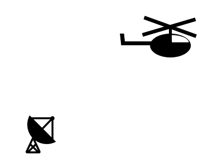
Consider a helicopter with four rotor blades. Assume the radar is located at the origin. Specify the location of the helicopter as (500, 0, 500), which sets its distance away from the radar in meters and a velocity of (60, 0, 0) m/s.

radarpos = [0;0;0];
radarvel = [0;0;0];

tgtinitpos = [500;0;500];
tgtvel     = [60;0;0];
tgtmotion  = phased.Platform('InitialPosition',tgtinitpos,'Velocity',tgtvel);

In this simulation, the helicopter is modeled by five scatterers: the rotation center and the tips of four blades. The rotation center moves with the helicopter body. Each blade tip is 90 degrees apart from the tip of its neighboring blades. The blades are rotating at a constant speed of 4 revolutions per second. The arm length of each blade is 6.5 meters.

Nblades   = 4;
bladeang  = (0:Nblades-1)*2*pi/Nblades;
bladelen  = 6.5;
bladerate = deg2rad(4*360);  % rps -> rad/sec

All four blade tips are assumed to have identical reflectivities while the reflectivity for the rotation center is stronger.

c  = 3e8;
fc = 5e9;
helicop = phased.RadarTarget('MeanRCS',[10 .1 .1 .1 .1],'PropagationSpeed',c,...
    'OperatingFrequency',fc);

Helicopter Echo Simulation

Assume the radar operates at 5 GHz with a simple pulse. The pulse repetition frequency is 20 kHz. For simplicity, assume the signal propagates in free space.

fs     = 1e6;
prf    = 2e4;
lambda = c/fc;

wav = phased.RectangularWaveform('SampleRate',fs,'PulseWidth',2e-6,'PRF',prf);
ura = phased.URA('Size',4,'ElementSpacing',lambda/2);
tx  = phased.Transmitter;
rx  = phased.ReceiverPreamp;
env = phased.FreeSpace('PropagationSpeed',c,'OperatingFrequency',fc,...
    'TwoWayPropagation',true,'SampleRate',fs);
txant = phased.Radiator('Sensor',ura,'PropagationSpeed',c,'OperatingFrequency',fc);
rxant = phased.Collector('Sensor',ura,'PropagationSpeed',c,'OperatingFrequency',fc);

At each pulse, the helicopter moves along its trajectory. Meanwhile, the blades keep rotating, and the tips of the blades introduce additional displacement and angular speed.

NSampPerPulse = round(fs/prf);
Niter = 1e4;
y     = complex(zeros(NSampPerPulse,Niter));
rng(2018);
for m = 1:Niter
    % update helicopter motion
    t = (m-1)/prf;
    [scatterpos,scattervel,scatterang] = helicopmotion(t,tgtmotion,bladeang,bladelen,bladerate);

    % simulate echo
    x  = txant(tx(wav()),scatterang);                    % transmit
    xt = env(x,radarpos,scatterpos,radarvel,scattervel); % propagates to/from scatterers
    xt = helicop(xt);                                    % reflect
    xr = rx(rxant(xt,scatterang));                       % receive
    y(:,m) = sum(xr,2);                                  % beamform
end

This figure shows the range-Doppler response using the first 128 pulses of the received signal. You can see the display of three returns at the target range of approximately 700 meters.

rdresp  = phased.RangeDopplerResponse('PropagationSpeed',c,'SampleRate',fs,...
    'DopplerFFTLengthSource','Property','DopplerFFTLength',128,'DopplerOutput','Speed',...
    'OperatingFrequency',fc);
mfcoeff = getMatchedFilter(wav);
plotResponse(rdresp,y(:,1:128),mfcoeff);
ylim([0 3000])

While the returns look as though they are from different targets, they are actually all from the same target. The center return is from the rotation center, and is much stronger compared to the other two returns. This intensity is because the reflection is stronger from the helicopter body when compared to the blade tips. The plot shows a speed of -40 m/s for the rotation center. This value matches the truth of the target radial speed.

tgtpos = scatterpos(:,1);
tgtvel = scattervel(:,1);
tgtvel_truth = radialspeed(tgtpos,tgtvel,radarpos,radarvel)

tgtvel_truth =

  -43.6435

The other two returns are from the tips of the blades when they approach or depart the target at maximum speed. From the plot, the speeds corresponding to these two approach and depart detections are about 75 m/s and -160 m/s, respectively.

maxbladetipvel = [bladelen*bladerate;0;0];
vtp = radialspeed(tgtpos,-maxbladetipvel+tgtvel,radarpos,radarvel)
vtn = radialspeed(tgtpos,maxbladetipvel+tgtvel,radarpos,radarvel)

vtp =

   75.1853


vtn =

 -162.4723

You can associate all three detections to the same target via further processing, but that topic is beyond the scope of this example.

Blade Return Micro-Doppler Analysis

The time-frequency representation of micro-Doppler effects can reveal more information. This code constructs a time-frequency representation in the detected target range bin.

mf  = phased.MatchedFilter('Coefficients',mfcoeff);
ymf = mf(y);
[~,ridx] = max(sum(abs(ymf),2)); % detection via peak finding along range
pspectrum(ymf(ridx,:),prf,'spectrogram')

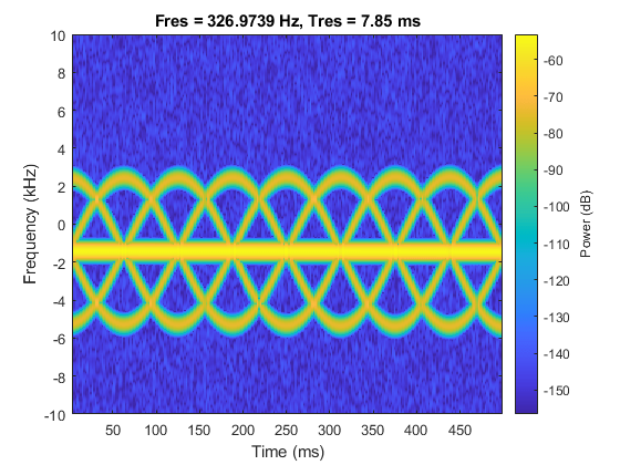
The figure shows the micro-Doppler modulation caused by blade tips around a constant Doppler shift. The image suggests that each blade tip introduces a sinusoid-like Doppler modulation. As noted in the figure below, within each period of the sinusoid, there are three extra sinusoids appearing at equal distance. This appearance suggests that the helicopter is equipped with four equally spaced blades.

hanno = helperAnnotateMicroDopplerSpectrogram(gcf);

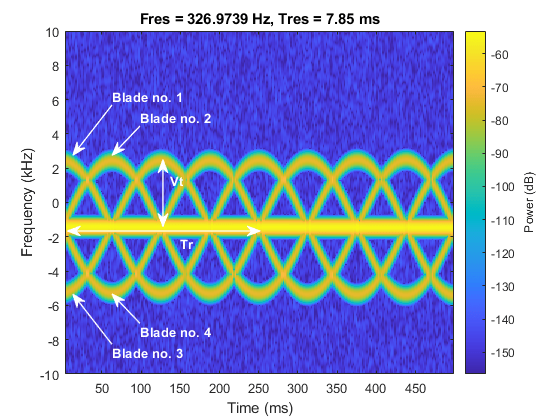
In addition to the number of blades, the image also shows that the period of each sinusoid, Tr, is about 250 ms. This value means that a blade returns to its original position after 250 ms. In this case, the angular speed of the helicopter is about 4 revolutions per second, which matches the simulation parameter.

Tp = 250e-3;
bladerate_est = 1/Tp

bladerate_est =

     4

This image also shows the tip velocity Vt, which can be derived from the maximum Doppler. The maximum Doppler is about 4 kHz away from the constant Doppler introduced by the bulk movement. Calculate the detected maximum tip velocity.

Vt_detect = dop2speed(4e3,c/fc)/2

Vt_detect =

   120

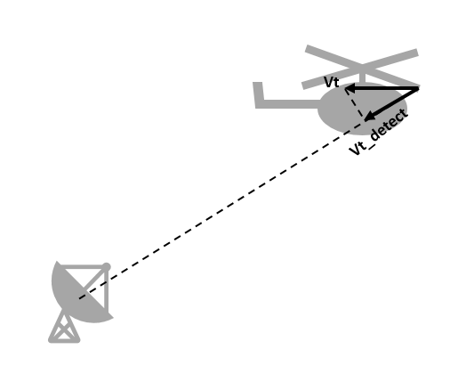
This value is the maximum tip velocity along the radial direction. To obtain the correct maximum tip velocity, the relative orientation must be taken into consideration. Because the blades are spinning in a circle, the detection is not affected by the azimuth angle. Correct only the elevation angle for the maximum tip velocity result.

doa = phased.MUSICEstimator2D('SensorArray',ura,'OperatingFrequency',fc,...
    'PropagationSpeed',c,'DOAOutputPort',true,'ElevationScanAngles',-90:90);
[~,ang_est] = doa(xr);
Vt_est = Vt_detect/cosd(ang_est(2))

Vt_est =

  164.0793

Based on the corrected maximum tip velocity and the blade-spinning rate, calculate the blade length.

bladelen_est = Vt_est/(bladerate_est*2*pi)

bladelen_est =

    6.5285

Note that the result matches the simulation parameter of 6.5 meters. Information such as number of blades, blade length, and blade rotation rate can help identify the model of the helicopter.

Pedestrian Identification in Automotive Radar

Considering an ego car with an FMCW automotive radar system whose bandwidth is 250 MHz and operates at 24 GHz.

bw = 250e6;
fs = bw;
fc = 24e9;
tm = 1e-6;
wav = phased.FMCWWaveform('SampleRate',fs,'SweepTime',tm,...
    'SweepBandwidth',bw);

The ego car is traveling along the road. Along the way, there is a car parked on the side of street and a human is walking out behind the car. The scene is illustrated in the following diagram

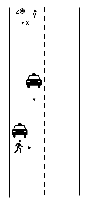
Based on this setup, if the ego car cannot identify that a pedestrian is present, an accident may occur.

egocar_pos = [0;0;0];
egocar_vel = [30*1600/3600;0;0];
egocar = phased.Platform('InitialPosition',egocar_pos,'Velocity',egocar_vel,...
    'OrientationAxesOutputPort',true);

parkedcar_pos = [39;-4;0];
parkedcar_vel = [0;0;0];
parkedcar = phased.Platform('InitialPosition',parkedcar_pos,'Velocity',parkedcar_vel,...
    'OrientationAxesOutputPort',true);
parkedcar_tgt = phased.RadarTarget('PropagationSpeed',c,'OperatingFrequency',fc,'MeanRCS',10);

ped_pos = [40;-3;0];
ped_vel = [0;1;0];
ped_heading = 90;
ped_height = 1.8;
ped = phased.BackscatterPedestrian('InitialPosition',ped_pos,'InitialHeading',ped_heading,...
    'PropagationSpeed',c,'OperatingFrequency',fc,'Height',1.6,'WalkingSpeed',1);

chan_ped = phased.FreeSpace('PropagationSpeed',c,'OperatingFrequency',fc,...
    'TwoWayPropagation',true,'SampleRate',fs);
chan_pcar = phased.FreeSpace('PropagationSpeed',c,'OperatingFrequency',fc,...
    'TwoWayPropagation',true,'SampleRate',fs);

tx = phased.Transmitter('PeakPower',1,'Gain',25);
rx = phased.ReceiverPreamp('Gain',25,'NoiseFigure',10);

Pedestrian Micro-Doppler Extraction

The following figure shows the range-Doppler map generated from the ego car's radar over time. Because the parked car is a much stronger target than the pedestrian, the pedestrian is easily shadowed by the parked car in the range-Doppler map. As a result, the map always shows a single target.

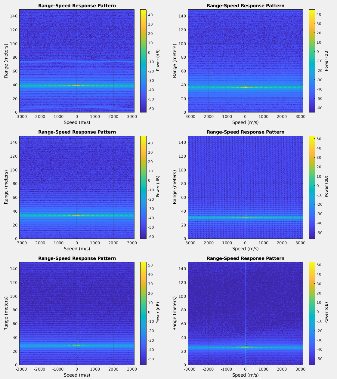
This means that conventional processing cannot satisfy our needs under this situation.

Micro-Doppler effect in time frequency domain can be a good candidate to identify if there is pedestrian signature embedded in the radar signal. As an example, the following section simulates the radar return for 2.5 seconds.

Tsamp = 0.001;
npulse = 2500;
xr = complex(zeros(round(fs*tm),npulse));
xr_ped = complex(zeros(round(fs*tm),npulse));
for m = 1:npulse
    [pos_ego,vel_ego,ax_ego] = egocar(Tsamp);
    [pos_pcar,vel_pcar,ax_pcar] = parkedcar(Tsamp);
    [pos_ped,vel_ped,ax_ped] = move(ped,Tsamp,ped_heading);
    [~,angrt_ped] = rangeangle(pos_ego,pos_ped,ax_ped);
    [~,angrt_pcar] = rangeangle(pos_ego,pos_pcar,ax_pcar);

    x = tx(wav());
    xt_ped = chan_ped(repmat(x,1,size(pos_ped,2)),pos_ego,pos_ped,vel_ego,vel_ped);
    xt_pcar = chan_pcar(x,pos_ego,pos_pcar,vel_ego,vel_pcar);
    xt_ped = reflect(ped,xt_ped,angrt_ped);
    xt_pcar = parkedcar_tgt(xt_pcar);
    xr_ped(:,m) = rx(xt_ped);
    xr(:,m) = rx(xt_ped+xt_pcar);
end

xd_ped = conj(dechirp(xr_ped,x));
xd = conj(dechirp(xr,x));

In the simulated signal, xd_ped contains only the pedestrian's return while xd contains the return from both the pedestrian and the parked car. If we generate a spectrogram using only the return of the pedestrian, we obtain a plot shown below.

clf;
spectrogram(sum(xd_ped),kaiser(128,10),120,256,1/Tsamp,'centered','yaxis');
clim = get(gca,'CLim');
set(gca,'CLim',clim(2)+[-50 0])

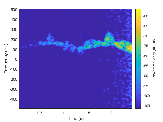
Note that the swing of arms and legs produces many parabolic curves in the time frequency domain along the way. Therefore such features can be used to determine whether a pedestrian exists in the scene.

However, when we generate a spectrogram directly from the total return, we get the following plot.

spectrogram(sum(xd),kaiser(128,10),120,256,1/Tsamp,'centered','yaxis');
clim = get(gca,'CLim');
set(gca,'CLim',clim(2)+[-50 0])

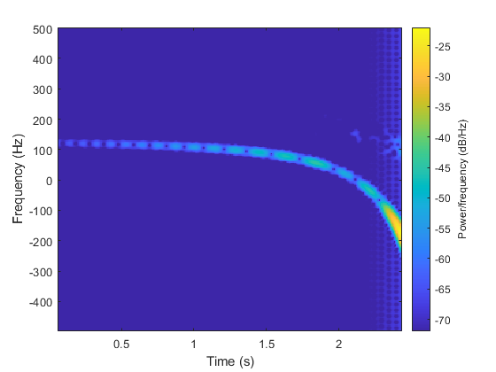
What we observe is that the parked car's return continue dominating the return, even in the time frequency domain. Therefore the time frequency response shows only the Doppler relative to the parked car. The drop of the Doppler frequency is due to the ego car getting closer to the parked car and the relative speed drops towards 0.

To see if there is a return hidden behind the strong return, we can use the singular value decomposition. The following plot shows the distribution of the singular value of the dechirped pulses.

[uxd,sxd,vxd] = svd(xd);
clf
plot(10*log10(diag(sxd)));
xlabel('Rank');
ylabel('Singular Values');
hold on;
plot([56 56],[-40 10],'r--');
plot([100 100],[-40 10],'r--');
plot([110 110],[-40 10],'r--');
text(25,-10,'A');
text(75,-10,'B');
text(105,-10,'C');
text(175,-10,'D');

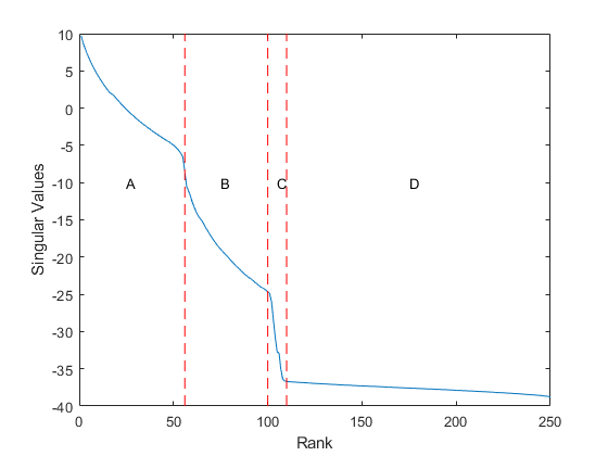
From the curve, it is clear that there are approximately four regions. The region A represents the most significant contribution to the signal, which is the parked car. The region D represents the noise. Therefore, the region B and C are due to the mix of parked car return and the pedestrian return. Because the return from the pedestrian is much weaker than the return from the parked car. In region B, it can still be masked by the residue of the return from the parked car. Therefore, we pick the region C to reconstruct the signal, and then plot the time frequency response again.

rk = 100:110;
xdr = uxd(:,rk)*sxd(rk,:)*vxd';
clf
spectrogram(sum(xdr),kaiser(128,10),120,256,1/Tsamp,'centered','yaxis');
clim = get(gca,'CLim');
set(gca,'CLim',clim(2)+[-50 0])

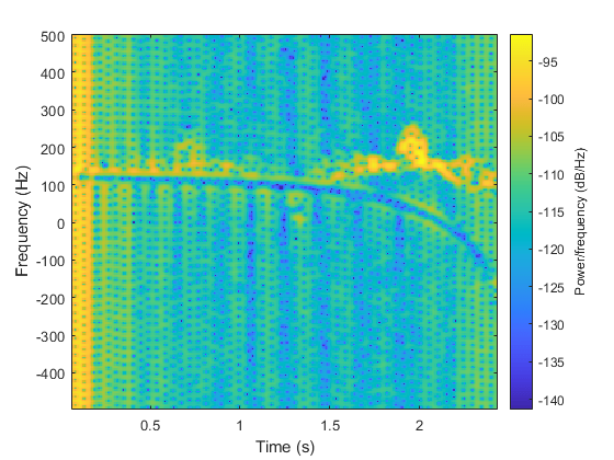
With the return from the car successfully filtered, the micro-Doppler signature from the pedestrian appears. Therefore, we can conclude that there is pedestrian in the scene and act accordingly to avoid an accident.

Summary

This example introduces the basic concept of a micro-Doppler effect and shows its impact on the target return. It also shows how to extract a micro-Doppler signature from the received I/Q signal and then derive relevant target parameters from the micro-Doppler information.

References

[1] Chen, V. C., The Micro-Doppler Effect in Radar, Artech House, 2011

[2] Chen, V. C., F. Li, S.-S. Ho, and H. Wechsler, "Micro-Doppler Effect in Radar: Phenomenon, Model, and Simulation Study", IEEE Transactions on Aerospace and Electronic Systems, Vol 42, No. 1, January 2006

Utility Functions

Function helicopmotion models the motion of multiple scatterers of the helicopter.

function [scatterpos,scattervel,scatterang] = helicopmotion(...
    t,tgtmotion,BladeAng,ArmLength,BladeRate)

prf = 2e4;
radarpos = [0;0;0];
Nblades  = size(BladeAng,2);

[tgtpos,tgtvel] = tgtmotion(1/prf);

RotAng     = BladeRate*t;
scatterpos = [0 ArmLength*cos(RotAng+BladeAng);0 ArmLength*sin(RotAng+BladeAng);zeros(1,Nblades+1)]+tgtpos;
scattervel = [0 -BladeRate*ArmLength*sin(RotAng+BladeAng);...
    0 BladeRate*ArmLength*cos(RotAng+BladeAng);zeros(1,Nblades+1)]+tgtvel;

[~,scatterang] = rangeangle(scatterpos,radarpos);

end