Introduction

Pd is the probability of saying that 1 is true given that event 1 occurred. Pfa is the probability of saying that 1 is true given that the 0 event occurred. In applications such as sonar and radar, the 1 event indicates that a target is present, and the 0 event indicates that a target is not present.

The performance of a detector is measured by its ability to achieve a certain Pd and Pfa for a given SNR. Examining the ROC curves provides insight into its performance. You can use the rocsnr function to calculate and plot the ROC curves.

Single Pulse Detection

Given an SNR value, you can calculate the Pd and Pfa values that a linear or square-law detector can achieve using a single pulse. Set the Pd value assuming that you have an SNR value of 8 dB and the requirements dictate a Pfa value of at most 1%. You can use the rocsnr function to calculate the Pd and Pfa values and then determine what value of Pd corresponds to Pfa = 0.01. Note that by default the rocsnr function assumes coherent detection.

[Pd,Pfa] = rocsnr(8);
idx = find(Pfa==0.01); % find index for Pfa=0.01

Using the index determined above you can find the Pd value that corresponds to Pfa = 0.01.

Pd(idx)

ans = 0.8899

One feature of the rocsnr function is that you can specify a vector of SNR values and the function calculates the ROC curve for each of these SNR values. Instead of individually calculating Pd and Pfa values for a given SNR, your can view the results in a plot of ROC curves. The rocsnr function plots the ROC curves by default if no output arguments are specified. Calling the rocsnr function with an input vector of four SNR values and no output arguments produces a plot of the ROC curves.

SNRvals = [2 4 8 9.4];
rocsnr(SNRvals);

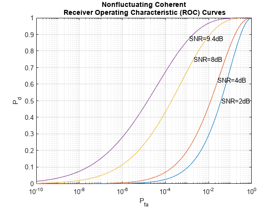
In the plot, select the data cursor button in the toolbar (or in the Tools menu) and then select the SNR = 8 dB curve at the point where Pd = 0.9 to verify that Pfa is approximately 0.01.

Multiple Pulse Detection

One way to improve detector performance is to average over several pulses. This is particularly useful in cases where the signal of interest is known and occurs in additive complex white noise. Although this still applies to both linear and square-law detectors, the result for square-law detectors could be off by about 0.2 dB. Analyze the performance by assuming an SNR of 8 dB and averaging over two pulses.

rocsnr(8,'NumPulses',2);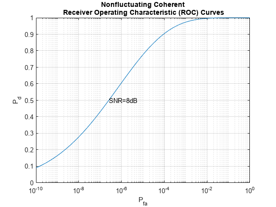

By inspecting the plot you can see that averaging over two pulses resulted in a higher probability of detection for a given false alarm rate. With an SNR of 8 dB and averaging over two pulses, you can constrain the probability of false alarm to be at most 0.0001 and achieve a probability of detection of 0.9. Recall that for a single pulse, you had to allow the probability of false alarm to be as much as 1% to achieve the same probability of detection.

Noncoherent Detector

To this point, the example deals with a known signal in complex white Gaussian noise. The rocsnr function by default assumes a coherent detector. To analyze the performance of a detector for the case where the signal is known except for the phase, you can specify a noncoherent detector. Using the same SNR values as before, analyze the performance of a noncoherent detector.

rocsnr(SNRvals,'SignalType','NonfluctuatingNoncoherent');

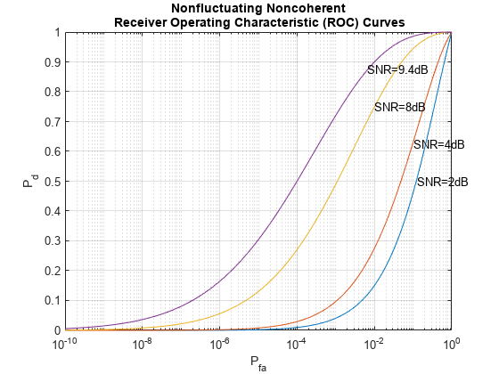
Focus on the ROC curve corresponding to an SNR of 8 dB. By inspecting the graph with the data cursor, you can see that to achieve a probability of detection of 0.9, you must tolerate a false-alarm probability of up to 0.05. Without using phase information, you will need a higher SNR to achieve the same Pd for a given Pfa. For noncoherent linear detectors, use Albersheim's equation to determine what value of SNR will achieve the desired Pd and Pfa.

SNR_valdB = albersheim(0.9,.01)  % Pd=0.9 and Pfa=0.01

SNR_valdB = 9.5027

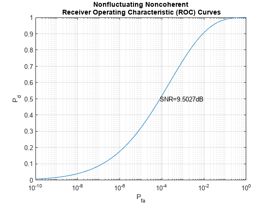
Plotting the ROC curve for the SNR value approximated by Albersheim's equation, you can see that the detector will achieve Pd = 0.9 and Pfa = 0.01. Note that the Albersheim's technique applies only to noncoherent detectors.

rocsnr(SNR_valdB,'SignalType','NonfluctuatingNoncoherent');

Detection of Fluctuating Targets

All the discussions above assume that the target is nonfluctuating, which means that the statistical characteristics of the target do not change over time. However, in real scenarios, targets can accelerate and decelerate as well as roll and pitch. These factors cause the radar cross section (RCS) of the target to vary over time. A set of statistical models called Swerling models are often used to describe the random variation in target RCS.

There are four Swerling models, namely Swerling 1 -- 4. The nonfluctuating target is often termed either Swerling 0 or Swerling 5. Each Swerling model describes how the RCS of a target varies over time and the probability distribution of the variation.

Because the target RCS is varying, the ROC curves for fluctuating targets are not the same as the nonfluctuating ones. In addition, because Swerling targets add random phase into the received signal, it is harder to use a coherent detector for a Swerling target. Therefore, noncoherent detection techniques are often used for Swerling targets.

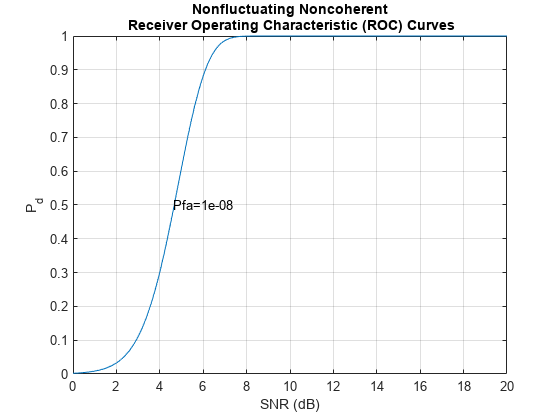
Now compare the ROC curves for a nonfluctuating target and a Swerling 1 target. In particular, you want to explore what the SNR requirements are for both situations if you want to achieve the same Pd and Pfa. For such a comparison, it is often easy to plot the ROC curve as Pd against SNR with varying Pfa. We can use the rocpfa function to plot the ROC curve in this form.

Assume noncoherent detection with 10 integrated pulses, with the desired Pfa being at most 1e-8. First, plot the ROC curve for a nonfluctuating target.

rocpfa(1e-8,'NumPulses',10,'SignalType','NonfluctuatingNoncoherent')

Then plot the ROC curve for a Swerling 1 target for comparison.

rocpfa(1e-8,'NumPulses',10,'SignalType','Swerling1')

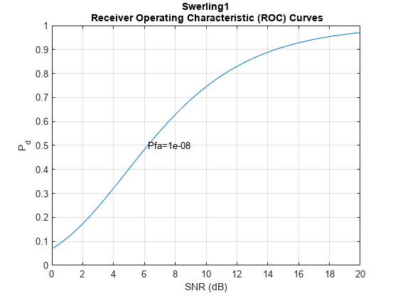
You can see from the figures, we can see that for a Pd of 0.9, you need an SNR of about 6 dB if the target is nonfluctuating. However, if the target is a Swerling case 1 model, the required SNR jumps to more than 14 dB, an 8 dB difference. This will greatly affect the design of the system.

As in the case of nonfluctuating targets, you have approximation equations to help determine the required SNR without having to plot all the curves. The equation used for fluctuating targets is Shnidman's equation. For the scenario used to plot the ROC curves, the SNR requirements can be derived using the shnidman function.

snr_sw1_db = shnidman(0.9,1e-8,10,1)  % Pd=0.9, Pfa=1e-8, 10 pulses, 

snr_sw1_db = 14.7131

                                      % Swerling case 1

The calculated SNR requirement matches the value derived from the curve.

Summary

ROC curves are useful for analyzing detector performance, both for coherent and noncoherent systems. This example used the rocsnr function to analyze the effectiveness of a linear detector for various SNR values. It also reviewed the improvement in detector performance achieved by averaging multiple samples. Lastly, the example showed how you can use the rocsnr and rocpfa functions to analyze detector performance when using a noncoherent detector for both nonfluctuating and fluctuating targets.