FMCW Waveform

Consider an automotive long range radar (LRR) used for adaptive cruise control (ACC). This kind of radar usually occupies the band around 77 GHz, as indicated in [1]. The radar system constantly estimates the distance between the vehicle it is mounted on and the vehicle in front of it, and alerts the driver when the two become too close. This figure shows a sketch of ACC.

A popular waveform used in ACC system is FMCW. The principle of range measurement using the FMCW technique can be illustrated using the following figure.

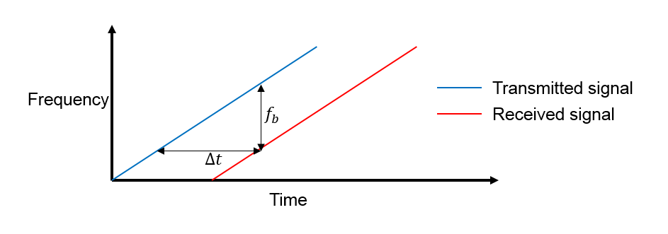
The received signal is a time-delayed copy of the transmitted signal where the delay, , is related to the range. Because the signal is always sweeping through a frequency band, at any moment during the sweep, the frequency difference, , is a constant between the transmitted signal and the received signal. is usually called the beat frequency. Because the sweep is linear, you can derive the time delay from the beat frequency and then translate the delay to the range.

In an ACC setup, the maximum range the radar needs to monitor is around 200 m and the system needs to be able to distinguish two targets that are 1 meter apart. From these requirements, you can compute the waveform parameters.

fc = 77e9;
c = 3e8;
lambda = c/fc;

The sweep time can be computed based on the time needed for the signal to travel the unambiguous maximum range. In general, for an FMCW radar system, the sweep time should be at least five to six times the round trip time. This example uses a factor of 5.5.

range_max = 200;
tm = 5.5*range2time(range_max,c);

The sweep bandwidth can be determined according to the range resolution and the sweep slope is calculated using both sweep bandwidth and sweep time.

range_res = 1;
bw = rangeres2bw(range_res,c);
sweep_slope = bw/tm;

Because an FMCW signal often occupies a large bandwidth, setting the sample rate blindly to twice the bandwidth often stresses the capability of A/D converter hardware. To address this issue, you can often choose a lower sample rate. Consider two things here:

In this example, the beat frequency corresponding to the maximum range is as follows.

fr_max = range2beat(range_max,sweep_slope,c);

Because the maximum speed of a traveling car is about 230 km/h. Hence the maximum Doppler shift and the maximum beat frequency can be computed as

v_max = 230*1000/3600;
fd_max = speed2dop(2*v_max,lambda);
fb_max = fr_max+fd_max;

This example adopts a sample rate of the larger of twice the maximum beat frequency and the bandwidth.

fs = max(2*fb_max,bw);

The following table summarizes the radar parameters.

System parameters            Value
----------------------------------
Operating frequency (GHz)    77
Maximum target range (m)     200
Range resolution (m)         1
Maximum target speed (km/h)  230
Sweep time (microseconds)    7.33
Sweep bandwidth (MHz)        150
Maximum beat frequency (MHz) 27.30
Sample rate (MHz)            150

With this information, set up the FMCW waveform used in the radar system.

waveform = phased.FMCWWaveform('SweepTime',tm,'SweepBandwidth',bw, ...
    'SampleRate',fs);

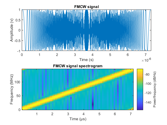
This is an up-sweep linear FMCW signal, often referred to as a sawtooth shape. Examine the time-frequency plot of the generated signal.

sig = waveform();
subplot(211); plot(0:1/fs:tm-1/fs,real(sig));
xlabel('Time (s)'); ylabel('Amplitude (v)');
title('FMCW signal'); axis tight;
subplot(212); spectrogram(sig,32,16,32,fs,'yaxis');
title('FMCW signal spectrogram');

Target Model

The target of an ACC radar is usually a car in front of it. This example assumes the target car is moving 43 m ahead of the car with the radar, at a speed of 96 km/h along the x-axis.

Compute the radar cross section of a car, according to [1], based on the distance between the radar and the target car.

car_dist = 43;
car_speed = 96*1000/3600;
car_rcs = db2pow(min(10*log10(car_dist)+5,20));
cartarget = phased.RadarTarget('MeanRCS',car_rcs,'PropagationSpeed',c,...
    'OperatingFrequency',fc);
carmotion = phased.Platform('InitialPosition',[car_dist;0;0.5],...
    'Velocity',[car_speed;0;0]);

Assume the propagation model to be free space.

channel = phased.FreeSpace('PropagationSpeed',c,...
    'OperatingFrequency',fc,'SampleRate',fs,'TwoWayPropagation',true);

Radar System Setup

The rest of the radar system includes the transmitter, the receiver, and the antenna. This example uses the parameters presented in [1]. Note that this example models only main components and omits the effect from other components, such as coupler and mixer. In addition, for the sake of simplicity, the antenna is assumed to be isotropic and the gain of the antenna is included in the transmitter and the receiver.

ant_aperture = 6.06e-4;                         % in square meter
ant_gain = aperture2gain(ant_aperture,lambda);  % in dB

tx_ppower = db2pow(5)*1e-3;                     % in watts
tx_gain = 9+ant_gain;                           % in dB

rx_gain = 15+ant_gain;                          % in dB
rx_nf = 4.5;                                    % in dB

transmitter = phased.Transmitter('PeakPower',tx_ppower,'Gain',tx_gain);
receiver = phased.ReceiverPreamp('Gain',rx_gain,'NoiseFigure',rx_nf,...
    'SampleRate',fs);

Automotive radars are generally mounted on vehicles, so they are often in motion. This example assumes the radar is traveling at a speed of 100 km/h along x-axis. So the target car is approaching the radar at a relative speed of 4 km/h.

radar_speed = 100*1000/3600;
radarmotion = phased.Platform('InitialPosition',[0;0;0.5],...
    'Velocity',[radar_speed;0;0]);

Radar Signal Simulation

As briefly mentioned in earlier sections, an FMCW radar measures the range by examining the beat frequency in the dechirped signal. To extract this frequency, a dechirp operation is performed by mixing the received signal with the transmitted signal. After the mixing, the dechirped signal contains only individual frequency components that correspond to the target range.

In addition, even though it is possible to extract the Doppler information from a single sweep, the Doppler shift is often extracted among several sweeps because within one pulse, the Doppler frequency is indistinguishable from the beat frequency. To measure the range and Doppler, an FMCW radar typically performs the following operations:

The next section simulates the process outlined above. A total of 64 sweeps are simulated and a range Doppler response is generated at the end.

During the simulation, a spectrum analyzer is used to show the spectrum of each received sweep as well as its dechirped counterpart.

specanalyzer = spectrumAnalyzer('SampleRate',fs, ...
    'Method','welch','AveragingMethod','running', ...
    'PlotAsTwoSidedSpectrum',true, 'FrequencyResolutionMethod','rbw', ...
    'Title','Spectrum for received and dechirped signal', ...
    'ShowLegend',true);

Next, run the simulation loop.

rng(2012);
Nsweep = 64;
xr = complex(zeros(waveform.SampleRate*waveform.SweepTime,Nsweep));

for m = 1:Nsweep
    % Update radar and target positions
    [radar_pos,radar_vel] = radarmotion(waveform.SweepTime);
    [tgt_pos,tgt_vel] = carmotion(waveform.SweepTime);

    % Transmit FMCW waveform
    sig = waveform();
    txsig = transmitter(sig);

    % Propagate the signal and reflect off the target
    txsig = channel(txsig,radar_pos,tgt_pos,radar_vel,tgt_vel);
    txsig = cartarget(txsig);

    % Dechirp the received radar return
    txsig = receiver(txsig);
    dechirpsig = dechirp(txsig,sig);

    % Visualize the spectrum
    specanalyzer([txsig dechirpsig]);

    xr(:,m) = dechirpsig;
end

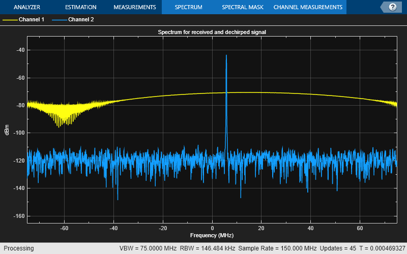
From the spectrum scope, you can see that although the received signal is wideband (channel 1), sweeping through the entire bandwidth, the dechirped signal becomes narrowband (channel 2).

Range and Doppler Estimation

Before estimating the value of the range and Doppler, take a look at the zoomed range Doppler response of all 64 sweeps.

rngdopresp = phased.RangeDopplerResponse('PropagationSpeed',c,...
    'DopplerOutput','Speed','OperatingFrequency',fc,'SampleRate',fs,...
    'RangeMethod','FFT','SweepSlope',sweep_slope,...
    'RangeFFTLengthSource','Property','RangeFFTLength',2048,...
    'DopplerFFTLengthSource','Property','DopplerFFTLength',256);

clf;
plotResponse(rngdopresp,xr);                     % Plot range Doppler map
axis([-v_max v_max 0 range_max])
climVals = clim;

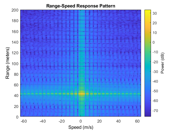
From the range Doppler response, you can see that the car in front is a bit more than 40 m away and appears almost static. This is expected because the radial speed of the car relative to the radar is only 4 km/h, which translates to a mere 1.11 m/s.

There are many ways to estimate the range and speed of the target car. For example, you can choose almost any spectral analysis method to extract both the beat frequency and the Doppler shift. This example uses the root MUSIC algorithm to extract both the beat frequency and the Doppler shift.

As a side note, although the received signal is sampled at 150 MHz so the system can achieve the required range resolution, after the dechirp, you need to sample it only at a rate that corresponds to the maximum beat frequency. Since the maximum beat frequency is in general less than the required sweeping bandwidth, the signal can be decimated to alleviate the hardware cost. The following code shows the decimation process.

Dn = fix(fs/(2*fb_max));
for m = size(xr,2):-1:1
    xr_d(:,m) = decimate(xr(:,m),Dn,'FIR');
end
fs_d = fs/Dn;

To estimate the range, firstly, estimate the beat frequency using the coherently integrated sweeps and then converted to the range.

fb_rng = rootmusic(pulsint(xr_d,'coherent'),1,fs_d);
rng_est = beat2range(fb_rng,sweep_slope,c)

rng_est =

   42.9976

Second, estimate the Doppler shift across the sweeps at the range where the target is present.

peak_loc = val2ind(rng_est,c/(fs_d*2));
fd = -rootmusic(xr_d(peak_loc,:),1,1/tm);
v_est = dop2speed(fd,lambda)/2

v_est =

    1.0830

Note that both range and Doppler estimation are quite accurate.

Range Doppler Coupling Effect

One issue associated with linear FM signals, such as an FMCW signal, is the range Doppler coupling effect. As discussed earlier, the target range corresponds to the beat frequency. Hence, an accurate range estimation depends on an accurate estimate of beat frequency. However, the presence of Doppler shift changes the beat frequency, resulting in a biased range estimation.

For the situation outlined in this example, the range error caused by the relative speed between the target and the radar is as follows

deltaR = rdcoupling(fd,sweep_slope,c)

deltaR =

   -0.0041

This error is so small that you can safely ignore it.

Even though the current design achieves the desired performance, one parameter warrants further attention. In the current configuration, the sweep time is about 7 microseconds. Therefore, the system needs to sweep a 150 MHz band within a very short period. Such an automotive radar might not be able to meet the cost requirement. Besides, given the velocity of a car, there is no need to make measurements every 7 microseconds. Hence, automotive radars often use a longer sweep time. For example, the waveform used in [2] has the same parameters as the waveform designed in this example except a sweep time of 2 ms.

A longer sweep time makes the range Doppler coupling more prominent. To see this effect, first reconfigure the waveform to use 2 ms as the sweep time.

waveform_tr = clone(waveform);
release(waveform_tr);
tm = 2e-3;
waveform_tr.SweepTime = tm;
sweep_slope = bw/tm;

Now calculate the range Doppler coupling.

deltaR = rdcoupling(fd,sweep_slope,c)

deltaR =

   -1.1118

A range error of 1.14 m can no longer be ignored and needs to be compensated. Naturally, you might consider doing so following the same procedure outlined in earlier sections, estimating both range and Doppler, figuring out the range Doppler coupling from the Doppler shift, and then remove the error from the estimate.

Unfortunately this process does not work very well with the long sweep time. The longer sweep time results in a lower sampling rate across the sweeps, thus reducing the capability of the radar for unambiguously detecting high speed vehicles. For instance, using a sweep time of 2 ms, the maximum unambiguous speed the radar system can detect using the traditional Doppler processing is as follows

v_unambiguous = dop2speed(1/(2*tm),lambda)/2

v_unambiguous =

    0.4870

The unambiguous speed is only 0.48 m/s, which means that the relative speed, 1.11 m/s, cannot be unambiguously detected. This means that not only the target car will appear slower in Doppler processing, but the range Doppler coupling also cannot be correctly compensated.

One way to resolve such ambiguity without Doppler processing is to adopt a triangle sweep pattern. Next section shows how the triangle sweep addresses the issue.

Triangular Sweep

In a triangular sweep, there is one up sweep and one down sweep to form one period, as shown in the following figure.

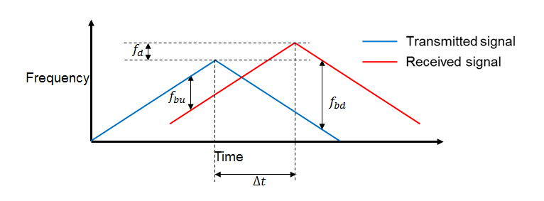
The two sweeps have the same slope except different signs. From the figure, you can see that the presence of Doppler frequency, , affects the beat frequencies ( and ) differently in up and down sweeps. Hence by combining the beat frequencies from both up and down sweep, the coupling effect from the Doppler can be averaged out and the range estimate can be obtained without ambiguity.

First, set the waveform to use triangular sweep.

waveform_tr.SweepDirection = 'Triangle';

Now simulate the signal return. Because of the longer sweep time, fewer sweeps (16 vs. 64) are collected before processing.

Nsweep = 16;
xr = helperFMCWSimulate(Nsweep,waveform_tr,radarmotion,carmotion,...
    transmitter,channel,cartarget,receiver);

The up sweep and down sweep are processed separately to obtain the beat frequencies corresponding to both up and down sweep.

fbu_rng = rootmusic(pulsint(xr(:,1:2:end),'coherent'),1,fs);
fbd_rng = rootmusic(pulsint(xr(:,2:2:end),'coherent'),1,fs);

Using both up sweep and down sweep beat frequencies simultaneously, the correct range estimate is obtained.

rng_est = beat2range([fbu_rng fbd_rng],sweep_slope,c)

rng_est =

   42.9658

Moreover, the Doppler shift and the velocity can also be recovered in a similar fashion.

fd = -(fbu_rng+fbd_rng)/2;
v_est = dop2speed(fd,lambda)/2

v_est =

    1.1114

The estimated range and velocity match the true values, 43 m and 1.11 m/s, very well.

Two-ray Propagation

To complete the discussion, in reality, the actual signal propagation between the radar and the target vehicle is more complicated than what is modeled so far. For example, the radio wave can also arrive at the target vehicle via reflections. A simple yet widely used model to describe such a multipath scenario is a two-ray model, where the signal propagates from the radar to the target vehicle via two paths, one direct path and one reflected path off the road, as shown in the following figure.

The reflection off the road affects the phase of the signal and the received signal at the target vehicle is a coherent combination of the signals via the two paths. The same thing happens on the return trip where the reflected signal from the target vehicle travels back to the radar. Hence depending on the distance between the vehicles, the signals from different paths may add constructively or destructively, making signal strength fluctuate over time. Such fluctuation can pose some challenge in the successive detection stage.

To showcase the multipath effect, next section uses the two-ray channel model to propagate the signal between the radar and the target vehicle.

txchannel = twoRayChannel('PropagationSpeed',c,...
    'OperatingFrequency',fc,'SampleRate',fs);
rxchannel = twoRayChannel('PropagationSpeed',c,...
    'OperatingFrequency',fc,'SampleRate',fs);
Nsweep = 64;
xr = helperFMCWTwoRaySimulate(Nsweep,waveform,radarmotion,carmotion,...
    transmitter,txchannel,rxchannel,cartarget,receiver);
plotResponse(rngdopresp,xr);                     % Plot range Doppler map
axis([-v_max v_max 0 range_max]);
clim(climVals);

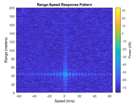
With all settings remaining same, the comparison of the resulting range-Doppler map with two-ray propagation and the range-Doppler map obtained before with a line of sight (LOS) propagation channel suggests that the signal strength dropped almost 40 dB, which is significant. Therefore, such effect must be considered during the design. One possible choice is to form a very sharp beam on the vertical direction to null out the reflections.

Summary

This example shows how to use FMCW signal to perform range and Doppler estimation in an automotive automatic cruise control application. The example also shows how to generate a range Doppler map from the received signal and how to use triangle sweep to compensate for the range Doppler coupling effect for the FMCW signal. Finally, the effect on the signal level due to the multipath propagation is discussed.

References

[1] Karnfelt, Camilla, et al. "77 GHz ACC Radar Simulation Platform." 2009 9th International Conference on Intelligent Transport Systems Telecommunications, (ITST), IEEE, 2009 , pp. 209–14. DOI.org (Crossref), https://doi.org/10.1109/ITST.2009.5399354.

[2] Rohling, H., and M. M. Meinecke. "Waveform Design Principles for Automotive Radar Systems." 2001 CIE International Conference on Radar Proceedings (Cat No.01TH8559) , IEEE, 2001, pp. 1–4. DOI.org (Crossref), https://doi.org/10.1109/ICR.2001.984612.