Introduction

To improve the signal to noise ratio (SNR), modern radar and sonar systems often employ the matched filter in the receiver chain. The ambiguity function of a waveform represents exactly the output of the matched filter when the specified waveform is used as the filter input. This exact representation makes the ambiguity function a popular tool for designing and analyzing waveforms. This approach provides an insight into the resolution capability in both delay and Doppler domains for a given waveform. Based on this analysis, one can then determine whether a waveform is suitable for a particular application.

The following sections use the ambiguity function to explore the range-Doppler relationship for several popular waveforms. To establish a comparison baseline, assume that the design specification of a radar system requires a maximum unambiguous range of 15 km and a range resolution of 150 m.

Rmax = 15e3;
Rres = 150;

Based on these design specifications, the pulse repetition frequency (PRF) and the bandwidth of the waveform can be computed as follows.

prf = 1/range2time(Rmax)

prf = 9.9931e+03

bw = rangeres2bw(Rres)

bw = 9.9931e+05

Rectangular Pulse Waveform

The simplest waveform is a rectangular waveform, sometimes also referred to as single frequency waveform. For the rectangular waveform, the pulse width is the reciprocal of the bandwidth.

A rectangular waveform can be created as follows.

tau = 1/bw;     % Pulse width
fs = 4*bw;      % Set the sampling frequency to a high value to generate smoother plots
rectwav = phased.RectangularWaveform('SampleRate',fs,'PRF',prf,'PulseWidth',tau)

rectwav = 
  phased.RectangularWaveform with properties:

                SampleRate: 3.9972e+06
     DurationSpecification: 'Pulse width'
                PulseWidth: 1.0007e-06
                       PRF: 9.9931e+03
     PRFSelectionInputPort: false
     FrequencyOffsetSource: 'Property'
           FrequencyOffset: 0
              OutputFormat: 'Pulses'
                 NumPulses: 1
             PRFOutputPort: false
    CoefficientsOutputPort: false

Because the analysis of a waveform is always performed on full pulses, keep the OutputFormat property as 'Pulses'. One can also check the bandwidth of the waveform using the bandwidth method.

rect_bw = bandwidth(rectwav)

rect_bw = 9.9931e+05

The resulting bandwidth matches the requirement. Now, generate one pulse of the waveform, and then examine it using the ambiguity function.

rectsamples = rectwav();
ambgfun(rectsamples,rectwav.SampleRate,rectwav.PRF)
xlim([-tau tau]*2e+6)

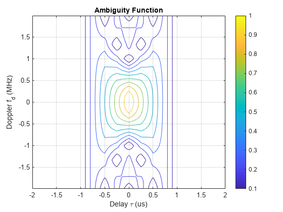
The nonzero response occupies only a small fraction of all delays focusing in a narrow strip around zero delay. This occurs because the waveform has a duty cycle of 0.01.

rect_dc = dutycycle(rectwav.PulseWidth,rectwav.PRF)

rect_dc = 0.0100

When investigating a waveform's resolution capability, the zero-delay cut and the zero-Doppler cut of the waveform ambiguity function are often of interest.

The zero-Doppler cut of the ambiguity function returns the auto-correlation function (ACF) of the rectangular waveform. The cut can be plotted using the following command.

ambgfun(rectsamples,rectwav.SampleRate,rectwav.PRF,'Cut','Doppler')
xlim([-tau tau]*2e+6)

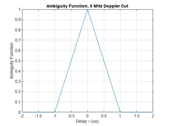
The zero-Doppler cut of the ambiguity function depicts the matched filter response of a target when the target is stationary. From the plot, one can see that the first null response appears at 1 microsecond, which means that this waveform is guaranteed to be able to resolve two targets that are at least 1 microsecond, or 150 m apart. Hence, the response matches the requirement in the design specification.

The zero-delay cut can be plotted using a similar syntax.

ambgfun(rectsamples,rectwav.SampleRate,rectwav.PRF,'Cut','Delay')
xlim([-bw bw]*2e-6)

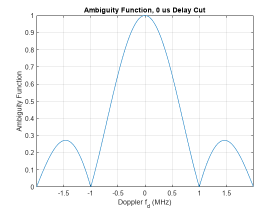
Notice that the returned zero-delay response is fairly broad. The first null appears at a Doppler shift of 1 MHz. Thus, if the two targets are at the same range, they need to have a difference of 1 MHz in the Doppler domain to be separated. Assuming the radar is working at 1 GHz, according to the computation below, such a separation corresponds to a speed difference of almost 150 km/s. Because this number is so large, essentially one cannot separate two targets in the Doppler domain using this system.

fc = 1e9;
rect_deltav = dop2speed(1e6,freq2wavelen(fc))/2

rect_deltav = 1.4990e+05

Another issue with the rectangular waveform is that the range resolution is determined by the pulse width. Thus, to achieve good range resolution, the system needs to adopt a very small pulse width. At the same time, the system also needs to be able to send out enough energy to the space so that the returned echo can be reliably detected. Hence, a narrow pulse width requires very high peak power at the transmitter. In practice, producing such power can be very costly.

Linear FM Pulse Waveform

One can see from the previous section that a single rectangular pulse has poor Doppler resolution. In fact, the Doppler resolution of a single rectangular pulse is given by the reciprocal of the pulse width. At the same time, the range resolution of a rectangular waveform is proportional to the pulse width. Apparently, there exists a conflict between range and Doppler resolutions of a rectangular waveform.

The root issue here is that both the delay and the Doppler resolution depend on the pulse width in opposite ways. Therefore, one way to solve this issue is to come up with a waveform that decouples this dependency. One can then improve the resolution in both domains simultaneously.

Linear FM waveform is just such a waveform. The range resolution of a linear FM waveform no longer depends on the pulse width. Instead, the range resolution is determined by the sweep bandwidth.

A system that transmits a linear FM waveform can afford a longer pulse width, which alleviates the power requirement. The longer pulse width also improves the Doppler resolution. This improvement occurs even though the Doppler resolution of a linear FM waveform is still given by the reciprocal of the pulse width.

Now, explore the linear FM waveform in detail. The linear FM waveform that provides the desired range resolution can be constructed as follows.

tau_fm = 50/bw;
lfmwav = phased.LinearFMWaveform('SampleRate',fs,'SweepBandwidth',bw,'PRF',prf,'PulseWidth',tau_fm)

lfmwav = 
  phased.LinearFMWaveform with properties:

                SampleRate: 3.9972e+06
     DurationSpecification: 'Pulse width'
                PulseWidth: 5.0035e-05
                       PRF: 9.9931e+03
     PRFSelectionInputPort: false
            SweepBandwidth: 9.9931e+05
            SweepDirection: 'Up'
             SweepInterval: 'Positive'
                  Envelope: 'Rectangular'
     FrequencyOffsetSource: 'Property'
           FrequencyOffset: 0
              OutputFormat: 'Pulses'
                 NumPulses: 1
             PRFOutputPort: false
    CoefficientsOutputPort: false

The pulse width of this linear FM waveform is 50 times longer than that of the rectangular waveform used in the earlier sections of this example. This means that the duty cycle is 50 times larger.

lfm_dc = dutycycle(lfmwav.PulseWidth,lfmwav.PRF)

lfm_dc = 0.5000

Notice that the bandwidth of the linear FM waveform is the same as the rectangular waveform.

lfm_bw = bandwidth(lfmwav)

lfm_bw = 9.9931e+05

The zero-Doppler cut of the ambiguity function for the linear FM waveform appears in the next plot. To better visualize the sidelobe behavior the ambiguity function is plotted in dB scale.

lfmsamples = lfmwav();
[lfmaf_delay,delay] = ambgfun(lfmsamples,lfmwav.SampleRate,lfmwav.PRF,'Cut','Doppler');

figure
hold on
plot(delay*1e6,mag2db(lfmaf_delay))
yline(-13.2,'Label','Sidelobe Level (-13.2 dB)')
grid on
xlabel('Delay \tau (us)')
ylabel('Ambiguity Function (dB)')
xlim([-tau_fm tau_fm]*3e5)
ylim([-50 0])
title('Ambiguity Function, 0 MHz Doppler Cut')

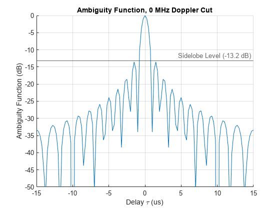
From the preceding figure, one can see that even though the response now has sidelobes, the first null still appears at 1 microsecond, so the range resolution is preserved. The sidelobe level for a waveform is often described using the peak-to-sidelobe ratio (PSR). Typically, the sidelobes near the main lobe are the highest. The sidelobes created by a stronger target can mask returns from a weaker target and make its detection impossible even if the two targets are resolvable in range. For a linear FM pulse with a rectangular amplitude the PSR is -13.2 dB.

One can also plot the zero-delay cut of the linear FM waveform. Observe that the first null in Doppler domain is now at around 20 kHz, which is 1/50 of the original rectangular waveform.

[lfmaf_doppler,doppler] = ambgfun(lfmsamples,lfmwav.SampleRate,lfmwav.PRF,'Cut','Delay');

figure
plot(doppler*1e-3,lfmaf_doppler)
grid on
xlabel('Doppler f_d (kHz)')
ylabel({'Ambiguity','Function'})
xlim([-200 200])
title('Ambiguity Function, 0 us Delay Cut')

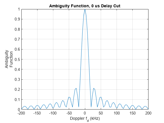
Following the same procedure as for the rectangular waveform in the earlier sections of this example, one can calculate that the 20 kHz Doppler separation translates to a speed difference of 3 km/s. This resolution is 50 times better than the rectangular waveform. Unfortunately, such resolution is still inadequate.

lfm_deltav = dop2speed(20e3,wavelen2freq(fc))/2

lfm_deltav = 2.9979e+03

It can be instructive to see a 3-D plot of the ambiguity function or to plot the top view of the ambiguity function as an image. To generate a plot in other than the contour format, you can just get the returned ambiguity function and then plot it using your favorite format. For example, the following snippet generates the surface plot and a top view image of a linear FM waveform ambiguity function.

[lfmaf,delay,doppler] = ambgfun(lfmsamples,lfmwav.SampleRate,lfmwav.PRF);

figure
tiledlayout(2, 1)

nexttile
surf(delay*1e6,doppler/1e3,lfmaf,'LineStyle','none')
xlim([-tau_fm tau_fm]*1e6)
ylim([-bw bw]*1e-3)
colorbar
view([-40,35])
xlabel('Delay \tau (us)')
ylabel('Doppler f_d (kHz)')

nexttile
imagesc(delay*1e6,doppler/1e3,mag2db(lfmaf))
xlim([-tau_fm tau_fm]*1e6)
ylim([-bw bw]*1e-3)
clim([-30 0])
cbar = colorbar;
cbar.Label.String = '(dB)';
axis xy
xlabel('Delay \tau (us)')
ylabel('Doppler f_d (kHz)')

sgtitle('Linear FM Pulse Waveform Ambiguity Function')

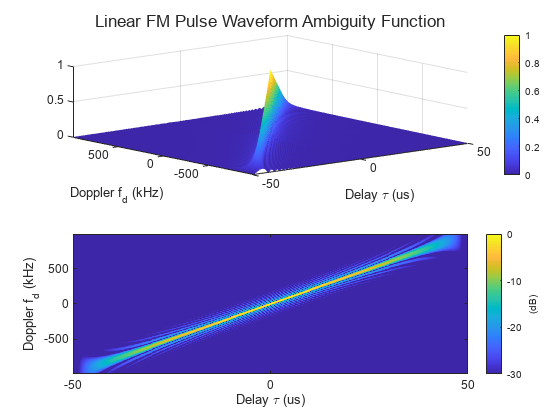
Notice that compared to the ambiguity function of the rectangular waveform, the ambiguity function of the linear FM waveform is tilted. This is due to delay-Doppler coupling. The tilt provides the improved resolution in the zero-delay cut.

Since typical Doppler shifts are much smaller compared to the waveform's bandwidth, the peak values of non-zero-Doppler cuts and hence the peak values of the matched filter outputs decrease only slightly when moving targets are observed. This behavior of the ambiguity function is what makes the linear FM waveform Doppler tolerant.

The ambiguity functions of both the rectangular waveform and the linear FM waveform have the shape of a long, narrow edge. This kind of ambiguity function is often termed as a knife edge ambiguity function.

Before proceeding to improve further the Doppler resolution, it is worth looking at an important figure of merit used in waveform analysis. The product of the pulse width and the bandwidth of a waveform is called the waveform's time-bandwidth product. For a rectangular waveform, the time-bandwidth product is always 1. For a linear FM waveform, because of the decoupling of the bandwidth and the pulse width, the time-bandwidth can be larger than 1. The waveform just used has a time-bandwidth product of 50. Recall that by preserving the same range resolution as the rectangular waveform, the linear FM waveform achieves a Doppler resolution that is 50 times better.

Coherent Pulse Train

As of the previous section, the Doppler resolution of the linear FM waveform is still fairly poor. One way to improve this resolution is to further extend the pulse width. However, this approach will not work for two reasons:

If one cannot extend the pulse width within one pulse, one has to look beyond this boundary. Indeed, in modern radar and sonar systems, the Doppler processing often uses a coherent pulse train. The more pulses in the pulse train, the finer the Doppler resolution.

To illustrate the idea, next, try a five-pulse burst.

release(lfmwav);
lfmwav.NumPulses = 5;
trainsamples = lfmwav();

First, plot the zero-Doppler cut of the ambiguity function.

[trainaf_delay,delay] = ambgfun(trainsamples,lfmwav.SampleRate,lfmwav.PRF,'Cut','Doppler');

figure
tiledlayout(2,1)

nexttile
plot(delay*1e6,trainaf_delay)
grid on
xlabel('Delay \tau (us)')
ylabel({'Ambiguity','Function'})
title('Ambiguity Function, 0 MHz Doppler Cut')

nexttile
plot(delay*1e6,trainaf_delay)
grid on
xlabel('Delay \tau (us)')
ylabel({'Ambiguity','Function'})
xlim([-2 2])

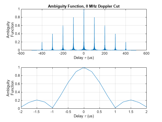
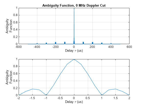
Notice that for the zero-Doppler cut, the first null is still around 1 microsecond, so the range resolution is the same. One should see immediately the presence of many range domain peaks. These peaks are the tradeoff for using a pulse train. The distance between the main lobe and the first peak is the length of one entire pulse, i.e., the reciprocal of the PRF.

T_max = 1/prf

T_max = 1.0007e-04

This time delay corresponds to the maximum unambiguous range.

The zero-delay cut also has peaks because of the pulse train.

[trainaf_doppler,doppler] = ambgfun(trainsamples,lfmwav.SampleRate,lfmwav.PRF,'Cut','Delay');

figure
tiledlayout(2,1)

nexttile
plot(doppler*1e-3,trainaf_doppler)
grid on
xlabel('Doppler f_d (kHz)')
ylabel({'Ambiguity','Function'})
title('Ambiguity Function, 0 us Delay Cut')
xlim([-bw bw]*1e-3)

nexttile
plot(doppler*1e-3,trainaf_doppler)
grid on
xlabel('Doppler f_d (kHz)')
ylabel({'Ambiguity','Function'})
xlim([-40 40])

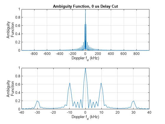
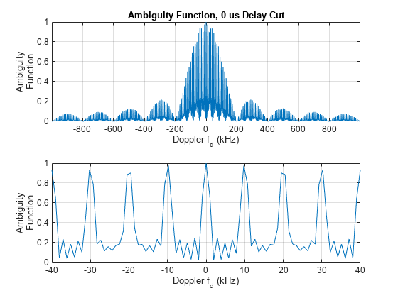
The distance between the adjacent peaks is equal to PRF. This value is the maximum unambiguous Doppler shift the system can measure. One can also calculate the corresponding maximum unambiguous speed.

V_max = dop2speed(lfmwav.PRF,freq2wavelen(fc))

V_max = 2.9959e+03

However, notice that the main lobe is now much sharper. Careful examination reveals that the first null is at about 2 kHz. This Doppler resolution can actually be obtained by the following equation,

train_deltaf = lfmwav.PRF/lfmwav.NumPulses

train_deltaf = 1.9986e+03

i.e., the resolution is now determined by the length of our entire pulse train, not the pulse width of a single pulse. The corresponding speed resolution is now

train_deltav = dop2speed(train_deltaf,freq2wavelen(fc))

train_deltav = 599.1701

which is significantly better. More importantly, to get even finer speed resolution, one can simply increase the number of pulses included in the pulse train. Of course, the number of pulses one can have in a burst depends on whether one can preserve the coherence for the entire duration, but that discussion is out of the scope of this example.

One may notice that in the zero-delay cut, the distance between the peaks is no longer constant, especially as the Doppler shift increases. This lack of constancy occurs because the linear FM waveform's ambiguity function is tilted. Hence, judging the separation of peaks in zero-delay cut can be misleading. The ambiguity caused by the pulse train is best observed from the top view, as the next code example shows. Notice that along the edge of the ambiguity function, those sidelobes are indeed evenly spaced.

[trainaf,delay,doppler] = ambgfun(trainsamples,lfmwav.SampleRate,lfmwav.PRF);

figure
tiledlayout(2, 1)

nexttile
imagesc(delay*1e6,doppler/1e3,mag2db(trainaf));
xlim([-1/prf 1/prf]*5e6)
ylim([-bw bw]*1e-3)
clim([-30 0])
cbar = colorbar;
cbar.Label.String = '(dB)';
axis xy
xlabel('Delay \tau (us)')
ylabel('Doppler f_d (kHz)')

nexttile
delay_idx = abs(delay) < 20e-6;
doppler_idx = abs(doppler) < 0.2e6;
contour(delay(delay_idx)*1e6,doppler(doppler_idx)/1e3,trainaf(doppler_idx,delay_idx))
xlabel('Delay \tau (us)')
ylabel('Doppler f_d (kHz)')
colorbar
grid on

sgtitle('Linear FM Pulse Train Waveform Ambiguity Function')

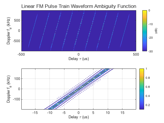
Because of all the peaks, this kind of ambiguity function is called a bed of nails ambiguity function.

Stepped FM Waveform

The linear FM waveform is very widely used in radar systems. However, it does present some challenges to the hardware. For one thing, the hardware has to be able to sweep the entire frequency range in one pulse. Using this waveform also makes it harder to build the receiver because it has to accommodate the entire bandwidth.

To avoid these issues, you can use a stepped FM waveform instead. A stepped FM waveform consists of multiple contiguous CW pulses. Each pulse has a different frequency and together, all pulses occupy the entire bandwidth. Hence, there is no more sweep within the pulse, and the receiver only needs to accommodate the bandwidth that is the reciprocal of the pulse width of a single pulse.

Next, set up such a stepped FM waveform.

stepfmwav = phased.SteppedFMWaveform('SampleRate', fs,'PulseWidth',5/bw,...
    'PRF',prf,'NumSteps',5,'FrequencyStep',bw/5,'NumPulses',5)

stepfmwav = 
  phased.SteppedFMWaveform with properties:

                SampleRate: 3.9972e+06
     DurationSpecification: 'Pulse width'
                PulseWidth: 5.0035e-06
                       PRF: 9.9931e+03
     PRFSelectionInputPort: false
             FrequencyStep: 1.9986e+05
                  NumSteps: 5
     FrequencyOffsetSource: 'Property'
           FrequencyOffset: 0
              OutputFormat: 'Pulses'
                 NumPulses: 5
             PRFOutputPort: false
    CoefficientsOutputPort: false

stepfmsamples = stepfmwav();

The zero-Doppler cut, zero-delay cut, and two-dimensional plot of the ambiguity function are shown below.

[stepaf_delay,delay] = ambgfun(stepfmsamples,stepfmwav.SampleRate,stepfmwav.PRF,'Cut','Doppler');

figure;
tiledlayout(2,1)

nexttile
plot(delay*1e6,stepaf_delay)
grid on
xlabel('Delay \tau (us)')
ylabel({'Ambiguity','Function'})
title('Ambiguity Function, 0 MHz Doppler Cut')

nexttile
plot(delay*1e6,stepaf_delay)
grid on
xlabel('Delay \tau (us)')
ylabel({'Ambiguity','Function'})
xlim([-2 2])

[stepaf_doppler,doppler] = ambgfun(stepfmsamples,stepfmwav.SampleRate,stepfmwav.PRF,'Cut','Delay');

figure
tiledlayout(2,1)

nexttile
plot(doppler*1e-3,stepaf_doppler)
grid on
xlabel('Doppler f_d (kHz)')
ylabel({'Ambiguity','Function'})
title('Ambiguity Function, 0 us Delay Cut')
xlim([-bw bw]*1e-3)

nexttile
plot(doppler*1e-3,stepaf_doppler)
grid on
xlabel('Doppler f_d (kHz)')
ylabel({'Ambiguity','Function'})
xlim([-40 40])

[stepaf,delay,doppler] = ambgfun(stepfmsamples,stepfmwav.SampleRate,stepfmwav.PRF);
 
figure
tiledlayout(2, 1)

nexttile
imagesc(delay*1e6,doppler/1e3,mag2db(stepaf)) 
xlim([-1/prf 1/prf]*5e6)
ylim([-bw bw]*1e-3)
clim([-30 0])
cbar = colorbar;
cbar.Label.String = '(dB)';
axis xy
xlabel('Delay \tau (us)')
ylabel('Doppler f_d (kHz)')

nexttile
delay_idx = abs(delay) < 20e-6;
doppler_idx = abs(doppler) < 0.2e6;
contour(delay(delay_idx)*1e6,doppler(doppler_idx)/1e3,stepaf(doppler_idx,delay_idx))
xlabel('Delay \tau (us)')
ylabel('Doppler f_d (kHz)')
colorbar
grid on

sgtitle('Stepped FM Waveform Ambiguity Function')

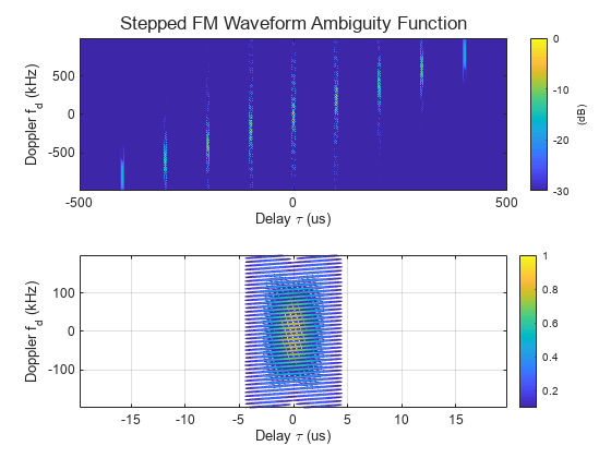
From these figures, one can make the following observations:

As to the disadvantage of a stepped FM waveform, the processing becomes more complicated.

Nonlinear FM Waveforms

Previous sections in this example showed that a linear FM pulse with a large time-bandwidth product can achieve a good resolution in range, while a coherent train of such pulses allows for achieving a good resolution in speed. Waveforms with large time-bandwidth products can also be generated by employing nonlinear FM. By selecting a particular nonlinear FM one can obtain a waveform with an ambiguity function that possesses some desired properties. For example, nonlinear FM can be used to obtain waveforms with low range sidelobes.

The shape of the waveform's spectrum determines the range sidelobe level. The spectrum of a linear FM pulse has an approximately rectangular shape. This is the reason the range sidelobes of a linear FM are 13.2 dB below the main lobe. Such relatively high sidelobe level might not be suited for some radar and sonar applications. The sidelobe level reduction can be accomplished by applying a window (taper) on the received side. The windowing, however, perturbs the matched filter result. Since the cumulative filtering no longer matches the signal exactly, it also reduces the output SNR. In contrast to linear FM, nonlinear FM waveforms can achieve low range sidelobes by shaping the spectrum using frequency modulation. In this case the time domain envelope remains constant and the loss in SNR is not incurred.

Various nonlinear functions can be used to modulate the instantaneous frequency of nonlinear FM waveforms. Often a nonlinear FM waveform is constructed by combining linear and nonlinear frequency modulation. For example, in [3] a hybrid nonlinear FM waveform is presented that is a combination of a linear and a tangent FM.

To construct a hybrid linear-tangent FM waveform two additional parameters must be specified. The first parameter, alpha, determines the balance between the linear and the tangent components. If alpha is zero, the resulting waveform will have only linear frequency modulation. If alpha is one, the instantaneous frequency of the resulting waveform will follow the tangent curve. The second parameter, gamma, determines the portion of the tangent curve that is used. By adjusting alpha and gamma the range sidelobes of the hybrid linear-tangent FM waveform can be made significantly lower than -13.2 dB, while keeping the range resolution close to the range resolution of the linear FM.

Create a hybrid linear-tangent FM waveform with the same pulse width, bandwidth, and PRF as the linear FM discussed in the earlier sections.

alpha = 0.5;
gamma = 1.4;
nlfmwav = phased.NonlinearFMWaveform('SampleRate',fs,'PulseWidth',tau_fm, ...
    'SweepBandwidth',bw,'FrequencyModulation','Hybrid Linear-Tangent', ...
    'LinearTangentBalance',alpha,'TangentCurvePortion',gamma,'PRF',prf)

nlfmwav = 
  phased.NonlinearFMWaveform with properties:

                SampleRate: 3.9972e+06
     DurationSpecification: 'Pulse width'
                PulseWidth: 5.0035e-05
                       PRF: 9.9931e+03
     PRFSelectionInputPort: false
       FrequencyModulation: 'Hybrid Linear-Tangent'
      LinearTangentBalance: 0.5000
       TangentCurvePortion: 1.4000
            SweepBandwidth: 9.9931e+05
            SweepDirection: 'Up'
             SweepInterval: 'Positive'
                  Envelope: 'Rectangular'
     FrequencyOffsetSource: 'Property'
           FrequencyOffset: 0
              OutputFormat: 'Pulses'
                 NumPulses: 1
             PRFOutputPort: false
    CoefficientsOutputPort: false

Compute and plot in the dB scale the zero-Doppler cut of the ambiguity function for the hybrid linear-tangent FM. For comparison show the corresponding zero-Doppler cut for the linear FM waveform.

nlfmsamples = nlfmwav();

[nlfmaf_delay, delay] = ambgfun(nlfmsamples,fs,prf,'Cut','Doppler');
 
figure
hold on
plot(delay*1e6,mag2db(lfmaf_delay),'--')
plot(delay*1e6,mag2db(nlfmaf_delay))
yline(-23.5,'Label','Sidelobe Level (-23.5 dB)')
grid on
xlabel('Delay \tau (us)')
ylabel({'Ambiguity Function (dB)'})
xlim([-tau_fm tau_fm]*3e5)
ylim([-50 0])
title('Ambiguity Function, 0 MHz Doppler Cut');
legend('Linear FM', 'Nonlinear FM')

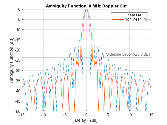
The zero-Doppler cut of the ambiguity function for the hybrid linear-tangent FM shows that the first null occurs at around 1.5 microseconds. This means that the range resolution is degraded to 225 m compared to 150 m for linear FM with the same bandwidth. The range sidelobe level, however, is more than 10 dB lower.

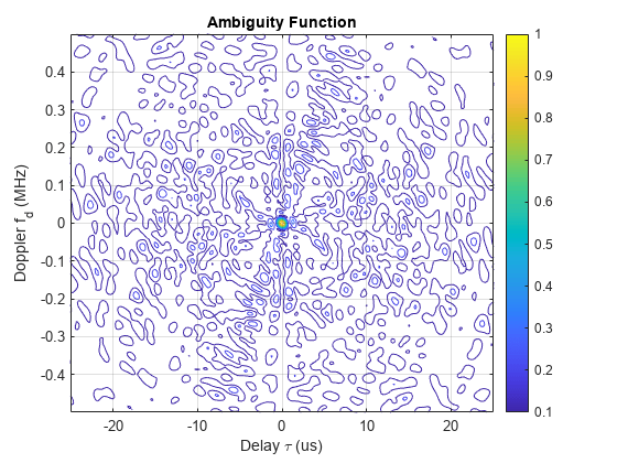
Nonlinear FM can also be used to generate a waveform with a thumbtack ambiguity function. An ideal thumbtack ambiguity function has a single sharp peak at the origin and a near-zero level everywhere else [1]. Waveforms with a thumbtack ambiguity are Doppler sensitive (Doppler intolerant) but can achieve high range and Doppler resolution. An example of a nonlinear FM that has a thumbtack ambiguity function is the generalized sinusoidal FM (GSFM) waveform [4]. The code below generates a GSFM waveform.

% Instantaneous frequency of a GSFM waveform
rho = 1.9;               % Variable exponent parameter
alpha = 1e9;             % Frequency modulation term
gsfm_finst = @(t)((bw/2)*sin(2*pi*alpha*t.^rho));
 
gsfmwav = phased.CustomFMWaveform('SampleRate',fs,...
    'PulseWidth',tau_fm,'FrequencyModulation',gsfm_finst,'PRF',prf)

gsfmwav = 
  phased.CustomFMWaveform with properties:

                SampleRate: 3.9972e+06
     DurationSpecification: 'Pulse width'
                PulseWidth: 5.0035e-05
                       PRF: 9.9931e+03
     PRFSelectionInputPort: false
       FrequencyModulation: @(t)((bw/2)*sin(2*pi*alpha*t.^rho))
                  Envelope: 'Rectangular'
     FrequencyOffsetSource: 'Property'
           FrequencyOffset: 0
              OutputFormat: 'Pulses'
                 NumPulses: 1
             PRFOutputPort: false
    CoefficientsOutputPort: false

gsfmsamples = gsfmwav();

The thumbtack nature of the ambiguity function with a single peak at the origin surrounded by low sidelobes is clearly visible in the contour plot.

figure
ambgfun(gsfmsamples,fs,prf)
xlim([-tau_fm tau_fm]*0.5e6)
ylim([-bw bw]*0.5e-6)

Barker-Coded Waveform

Another important group of waveforms is phase-coded waveforms, among which the popularly used ones are Barker codes, Frank codes, and Zadoff-Chu codes. In a phase-coded waveform, a pulse is divided into multiple subpulses, often referred to as chips, and each chip is modulated with a given phase. All phase-coded waveforms have good autocorrelation properties which make them good candidates for pulse compression. Thus, if a phase-coded waveform is adopted, it could lower the probability of interception as the energy is spread into chips. At the receiver, a properly configured matched filter could suppress the noise and achieve good range resolution.

Barker code is one of the most well-known phase-coded waveforms. A Barker-coded waveform can be constructed using the following command.

barkerwav = phased.PhaseCodedWaveform('Code','Barker','NumChips',7,...
    'SampleRate', fs,'ChipWidth',tau,'PRF',prf)

barkerwav = 
  phased.PhaseCodedWaveform with properties:

                SampleRate: 3.9972e+06
                      Code: 'Barker'
                 ChipWidth: 1.0007e-06
                  NumChips: 7
                       PRF: 9.9931e+03
     PRFSelectionInputPort: false
     FrequencyOffsetSource: 'Property'
           FrequencyOffset: 0
              OutputFormat: 'Pulses'
                 NumPulses: 1
             PRFOutputPort: false
    CoefficientsOutputPort: false

barkersamples = barkerwav();

This Barker code consists of 7 chips. Its zero-Doppler cut of the ambiguity function is given by

ambgfun(barkersamples,barkerwav.SampleRate,barkerwav.PRF,'Cut','Doppler')
xlim([-tau tau]*10e6)

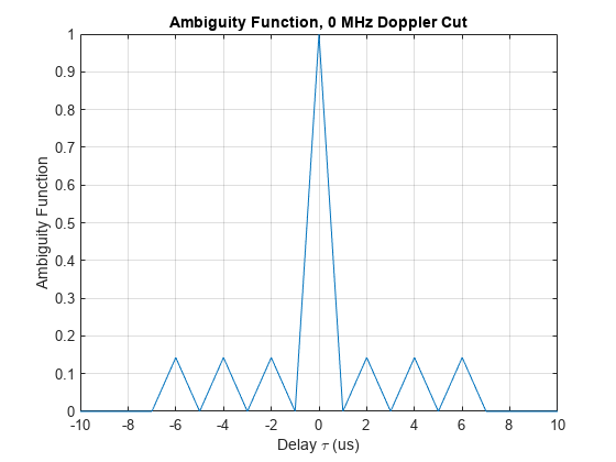
From the figure, one can see that the zero-Doppler cut of a Barker code's ambiguity function has an interesting property. All its sidelobes have the same height and are exactly 1/7 of the main lobe. In fact, a length-N Barker code can provide a peak-to-peak suppression of N, which helps distinguish closely located targets in range. This is the most important property of the Barker code. The range resolution is approximately 10 microseconds, the same as the chip width.

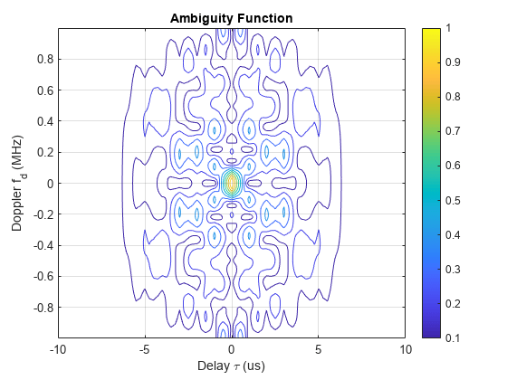
There are two issues associated with a Barker code. First, there are only seven known Barker codes. Their lengths are 2, 3, 4, 5, 7, 11 and 13. It is believed that there are no other Barker codes. Second, the Doppler performance of the Barker code is fairly poor. Although the ambiguity function has good shape at the zero-Doppler cut, once there is some Doppler shift, the sidelobe level increases significantly. Barker codes are Doppler sensitive with a thumbtack ambiguity function.

These properties of the Barker code are visible in the contour plot of the ambiguity function.

ambgfun(barkersamples,barkerwav.SampleRate,barkerwav.PRF)
xlim([-tau tau]*10e6)
ylim([-bw bw]*1e-6)

Summary

This example shows how to use the ambiguity function to analyze and compare waveforms. It compares several common waveforms including the rectangular waveform, the linear FM waveform, the stepped FM waveform, the hybrid linear-tangent FM waveform, the generalized sinusoidal FM waveform, and the Barker-coded waveform. The example shows that the ambiguity function is a convenient tool for analyzing Doppler tolerance of a waveform, its delay and Doppler resolution capabilities, and the sidelobe level.

Reference

[1] Nadav Levanon and Eli Mozeson, Radar Signals, Wiley-IEEE Press, 2004.

[2] Mark Richards, Fundamentals of Radar Signal Processing, McGraw Hill, 2005.

[3] Collins, T., and P. Atkins. "Nonlinear frequency modulation chirps for active sonar." IEE Proceedings-Radar, Sonar and Navigation 146.6 (1999): 312-316.

[4] Hague, David A., and John R. Buck. "The generalized sinusoidal frequency-modulated waveform for active sonar." IEEE Journal of Oceanic Engineering 42.1 (2016): 109-123.