Solve a Full Matrix System

First define the coefficient matrix $\mathit{A}$ as variable in the client memory, A, and then pass this matrix to the Creation function to create a distributed version of the same matrix, ADist. When you use the distributed function, MATLAB automatically starts a parallel pool using your default cluster settings.

n = 1e3;
A = randi(100,n,n);
ADist = distributed(A);

You can now define the right hand vector $$b$$. In this example, $$b$$ is defined as the row sum of $$A$$, which leads to an exact solution to $$Ax=b$$ of the form $$x_{\text{exact}}=[1,...,1{]}^T$$.

b = sum(A,2);
bDist = sum(ADist,2);

Since sum acts on a distributed array, bDist is also distributed and its data is stored in the memory of the workers of your parallel pool. Finally, define the exact solutions for comparison with the solutions obtained using direct numerical methods.

xEx = ones(n,1);
xDistEx = ones(n,1,'distributed');

Now that you have defined your system of linear equations, you can use mldivide to solve the system directly. In MATLAB, you can call mldivide using the special operator \. You do not have to change your code to solve the distributed system as mldivide has automatic support for distributed arrays.

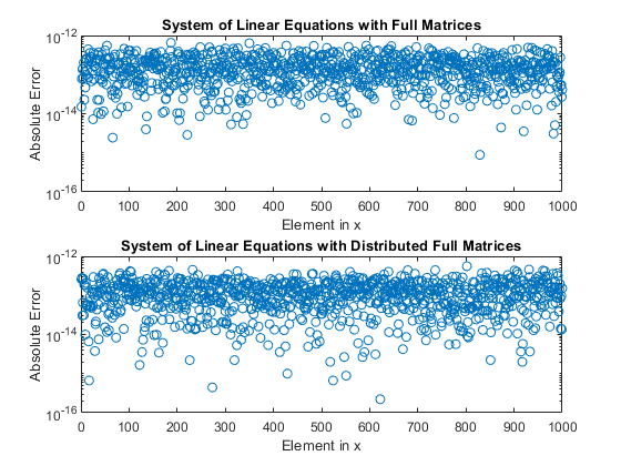
Once you have calculated the solution, you can check the error between each element of the obtained result $\mathit{x}$ and the expected values of $$x_{\text{exact}}$$.

x = A\b;
err = abs(xEx-x);

xDist = ADist\bDist;
errDist = abs(xDistEx-xDist);

figure
subplot(2,1,1)
semilogy(err,'o');
title('System of Linear Equations with Full Matrices');
ylabel('Absolute Error');
xlabel('Element in x');
ylim([10e-17,10e-13])
subplot(2,1,2)
semilogy(errDist,'o');
title('System of Linear Equations with Distributed Full Matrices');
ylabel('Absolute Error');
xlabel('Element in x');
ylim([10e-17,10e-13])

For both the distributed arrays and the arrays stored on the client, the absolute error between the calculated results for $\mathit{x}$ and the exact result $$x_{\text{exact}}$$ is small. The accuracy of the solution is approximately the same for both array types.

mean(err)

ans = 1.6031e-13

mean(errDist)

ans =

   1.2426e-13

Solve a Sparse Matrix System

Distributed arrays can also contain sparse data. To create the coefficient matrix $\mathit{A}$, use sprand and speye to directly generate a sparse matrix of random numbers plus the sparse identity matrix. Adding the identity matrix helps to prevent creating $\mathit{A}$ as a singular or near-singular matrix, both of which are difficult to factorize.

n = 1e3;
density = 0.2;
A = sprand(n,n,density) + speye(n);
ADist = distributed(A);

Choosing the right hand vector $$b$$ as the row sum of $$A$$ yields an exact solution of the same form as the solution to the full matrix system.

b = sum(A,2);
bDist = sum(ADist,2);
xEx = ones(n,1);
xDistEx = ones(n,1,'distributed');

In the same way as with full matrices, you can now solve this system of linear equations directly using mldivide and check the error between the obtained result and its expected value.

x = A\b;
err = abs(xEx-x);

xDist = ADist\bDist;
errDist = abs(xDistEx-xDist);

figure
subplot(2,1,1)
semilogy(err,'o');
title('System of Linear Equations with In-Client Sparse Matrices');
ylabel('Absolute Error');
xlabel('Element in x');
ylim([10e-17,10e-13])
subplot(2,1,2)
semilogy(errDist,'o');
title('System of Linear Equations with Distributed Sparse Matrices');
ylabel('Absolute Error');
xlabel('Element in x');
ylim([10e-17,10e-13])

As with the full matrix system, solving the system of linear equations using both on-client arrays and distributed arrays produces solutions with comparable accuracy.

mean(err)

ans = 1.6031e-13

mean(errDist)

ans =

   1.2426e-13

After you are done with your computations, you can delete your parallel pool. The gcp function returns the current parallel pool object so you can delete the current pool.

delete(gcp('nocreate'));

Improving Efficiency of the Solution

For certain types of large and sparse coefficient matrix $\mathit{A}$, there are more efficient methods than direct factorization for solving your systems. In these cases, iterative methods might be more efficient at solving your system of linear equations. Iterative methods generate a series of approximate solutions that converge to a final result. For an example of how to use iterative methods to solve linear equations with large, sparse input matrices, see Use Distributed Arrays to Solve Systems of Linear Equations with Iterative Methods.